The Once and Future Wallace

Real World Studies II: Stream Basins Morphometry.
A: Primary Tests.

     We have already seen from the simulations of randomly-generated four-class patterns on variously-shaped two-dimensional surfaces that a relatively small (but still some varying, depending in yet unknown ways on fineness of sampling grid and shape of boundary of system) proportion of these four-class patterns yield summary spatial autocorrelation statistics that when double-standardized yield the kind of symmetric z scores we are looking for here (all ij equal ji, all i equal j the same, all i equal j the largest z score in the matrix). We are now ready to look at the patterns produced by energy conditions in a variety of real world system which closely mirrors these simulations: stream drainage basins.

     Now technically speaking, we are not dealing with perfectly two-dimensional systems here: there is vertical range in the topographical component of any drainage basin, and beyond this the general curvature of the earth. Nevertheless, if one begins with relatively small systems the curvature complication becomes negligible (and in any case may be argued irrelevant on gravitational grounds), and in this instance the topography itself is the measured variable whose pattern in two dimensions is really what we are looking at. (For those who are still not convinced, I actually did run a parallel set of analyses to the ones described below in which I calculated distances between sample points not on the basis of their relative two-dimensional coordinates, but instead within three dimensions: sample point as intersecting the earth at x feet above sea level. The results differed only to the most trivial degree from the strictly two-dimensional ones.) What we are left with is a system comprised of areally distributed potential energies; that is, a "field" of varying elevations above sea level every location within which has a potential for doing work that is directly proportional to its elevation.

     In the case of the earth's internal zonation described in the last write-up, the four zones had evolved as a function of very large-scale forces exerted rather evenly and consistently over many millions, even billions, of years. Stream basins, however, are dynamic over a much shorter period of time and of course are less closed: with changes in sea level due to glaciation episodes or major tectonic events (or even local events such as stream piracy) energy conditions across any basin may change relatively rapidly. Thus, equilibrium within its surrounding environment may prove, even if it becomes possible under just the right conditions, fleeting. As a result, one finds few systems within which all portions of the basin are evenly balanced in terms of being exactly transitional between erosional and depositional environments.

     As we will see in the next write-up, the conditions of non-equilibrium within stream basins provide a number of potential secondary tests of the model under discussion here, but for the moment we will concentrate on the primary issue. If indeed the areal distribution of potential energies (elevations) within such systems can be interpreted through the model, we should expect that a(n efficient) classification of the elevations into four maximally-different ranges of elevation will yield patterns whose class-level spatial autocorrelation properties, again represented as a four by four matrix of values, will double-standardize into a symmetric arrangement of z scores. This should be true of all natural basins, though again, there is no initial reason to expect that our measures of equilibrium/redundancy (the mean r value of the correlation matrix for the spatial autocorrelation scores, and the total of the absolute values of the column means) should necessarily closely approach zero in value as they did for the earth zones model.

     In this instance there will be no a priori separation of zones as in that problem, so the zones must be derived. Here there is good reason for discussion as to what constitutes a proper approach to such derivation. I have begun with what seemed the most rational starting point: taking a regular triangular grid-based sample of elevations across each basin, ordering the resulting vector by heights, and then subjecting the resulting data to a nonhierarchical, information statistic-based clustering algorithm to identify its most efficient partitioning into four (or other number of) ranges of elevation values. Mapping the results of a given classification, we can see a pattern of classes that resembles a topographic map (the difference being that the isolines separating ranges of elevations are not necessarily spaced at equal intervals).

     [A methodological note: Those familiar with the use of information statistic-based nonhierarchical clustering algorithms are aware that the solutions are reached through an iterative process. This means they are prone to accidentally becoming "entrapped" within local minima, and reporting suboptimal results. The way around this problem is to initialize the process at a variety of starting configurations, and ultimately select the particular solution that accounts for the most variation in the data. In the many analyses I performed here (two- through six-class solutions for each of the twenty-five basins) this was done obsessively, to an extent that I am quite sure the solutions I accepted for further analysis were either the best ones outright, or very very close to them.]

     Once this basic plan of investigation was thought out, twenty-five drainage basins were chosen for examination. Over half of the basins selected were from northeastern United States 7.5 minute (1:24000) USGS quadrangle series maps, with the remainder from other U.S. areas and map series at various scales. Data collection was painfully manual, with transparent triangularly gridded overlays: each pinpointed sample location fell randomly between successive contour lines, requiring a careful act of interpolation to retrieve an actual (estimated) value. In this first round of studies, the number of points sampled varied from less than three hundred on the least sampled drainage basin to 550 on the most sampled one. These choices were a gamble: I figured that for an initial look at the matter a range of sources, geographical locations, and sample grid densities should be employed lest complaints be raised on this basis. However, it was unclear initially just how dense a sampling of the surfaces would be needed to reasonably capture the essence of the organization postulated.

     Table 1 provides basic stats on the basins studied:

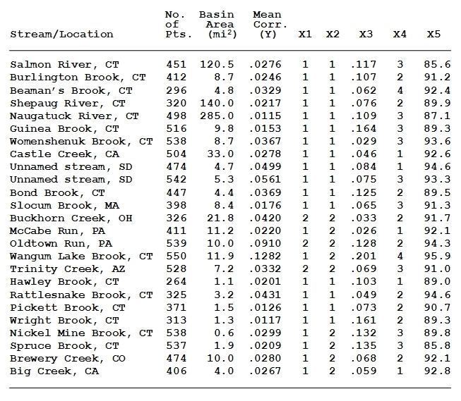
Table 1. Drainage basins used in the study. In the regression studies described in the next writeup, the dependent variable (Y) consists of the means of the correlation coefficients associated with each system's corresponding set of spatial autocorrelation scores; the X_i variables are: X1=whether the base map was derived from surface triangulation methods or aerial photography; X2=whether the base map used was the original map, or an nth generation copy thereof; X3=the standard deviations of the numbers of cases in each 4-class classification, converted to proportions of total; X4=a subjective rating of degree of vagueness of basin boundary; X5=the percentage of variation explained given by the n=4 nonhierarchical cluster analysis models.

     An example of the results of a sampling operation leading to a four-class classification, for Wright Brook, CT, is given here.

     Results? 24 of the 25 basins yielded double-standardized scores that were in fact symmetric in the sense anticipated. The one that didn't, "nearly converged" (especially after denser sampling was applied), but was the most problematic of the 25 to begin with because: (1) it was much the smallest basin looked at (only about 0.6 square miles in extent) (2) its drainage divides with surrounding basins were among the most poorly defined of the 25, and, most importantly, (3) ten or twenty percent of its area (per an on-site field check) had been artificially re-landscaped to support the building of a high school at the crest of a hill.

     Inasmuch as the basins studied included a wide variety of system sizes, and evolved under a considerable range of climate types and geologies, I have little doubt at this point that just about any such system, if sampled adequately, will yield the same results (though special cases such as karst landscapes and/or areas of internal drainage may present additional challenges to predictive modelling). This is pretty startling. It is, however, difficult or impossible to compare the results closely to any initial standard. The simulations I reported earlier that involved two-dimensional systems indicated that only a few percent of the patterns produced double-standardized results with the appropriate symmetrical Z scores condition, but these tests were run on variously-shaped areas and with several different numbers of sampled points, and through random assignment of classes, so a comparison of the actual systems to this standard is suggestive only.

     A further interesting discovery concerns the relative lack of variation among the arrays of z scores produced from the 25 analyses: most of them look pretty much like one another. Were much denser samplings of the basins taken, the resulting refinements in characterization of internal organization might well expose even greater similarities--and, conceivably, lack of variation altogether.

     As mentioned above, it should not be surprising to find here that, unlike the internal zonation patterns of the earth, there is no obvious division of each basin into four zones of elevation: simply, drainage basins are much more open systems that continually respond to all sorts of upsetting conditions that would prevent them from attaining conditions of dynamic equilibrium resulting in obvious, permanent, zonations. That said, however, a close enough look at a basin's organization might yet reveal some tendencies in that direction. As it turns out, this particular data set does exhibit evidence of such.

     First, there is the overall average of the mean r values connected with the correlation matrices for the twenty-five spatial autocorrelation matrices data that ultimately were double-standardized. In the two-dimensional simulations reported earlier, the mean r's across the eighteen groups of four-class solutions ranged from .029 to .198, with only one mean being below .050 (see the table in the 'Simulations: Two-Dimensional Systems' essay). Across the main (the first of the two "model #2" variations shown in Table 2 below) model for the twenty-five analyses reported here, the mean r values were: for three-class classifications of the sample elevations, .0572; for four-class classifications, .0348; for five-class classifications, .0326; and for six-class classifications, .0298. Notice, then, the rather lower mean for the four-class real world systems than for the simulated systems.

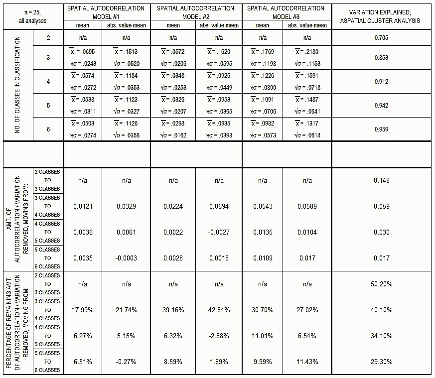
Table 2. Statistics comparing the spatial and aspatial models. See text for explanation.

     Table 2 presents the results of the analysis in greater detail, and these are worth going through more thoroughly. All the results shown in Table 2 pertain to mean values obtained across the twenty-five drainage basin tests. On the upper portion of the table the results of all three spatial autocorrelation analyses attempted are reported, along with the corresponding proportions of variation explained from the original cluster analyses; statistics are listed for two-class through six-class solutions (no spatial autocorrelation analyses were run on the two-class solutions, as the following entropy maximization operation leads to trivial results). For each spatial autocorrelation model, two sets of 25-case means (and their accompanying population standard deviations) are given, one connected to the mean column values of the correlation matrices derived from the twenty-five original spatial autocorrelation index matrices, the other to a corresponding mean value calculated from the absolute values of the column means (thus, deviation from a mean of zero, in either direction).

     The lower portion of Table 2 puts into better perspective the importance of the results obtained here. In the top half, the actual amount of reduction in the mean correlation/variation values as one increases the number of classes of elevations in the analyses. For example, for spatial autocorrelation model #2, "mean" for three-class classification is .0572, and for the four-class classification, .0348 (both as shown in the upper portion of Table 2); the difference is .0224, and this latter value appears in the corresponding spot in the top half of the lower portion of the table. In the column at the far right of the lower portion of the table, the number '0.148' appears; this corresponds to the increase in variation explained in the initial series of cluster analyses as one moves from the two-class analysis (.705) to the three-class one (.853). In the bottom half of the lower portion of Table 2, these values are translated into percentage improvements as the mean spatial autocorrelation values approach zero, and the variation explained approches 1.0. In the latter instance, and for example, the increase from a two-class to a three-class clustering model has absorbed just over fifty percent (50.20%) of the remaining variation (that is, .502 of the difference between 1.0 and .705, or .148).

     What all of this very clearly shows is that there is a clear difference between the spatial (spatial autocorrelation) and aspatial (nonhierarchical cluster analysis) models in terms of the pattern of reduction of unexplained variation as number of classes imposed increases. Over the twenty-five analyses, the pattern of increase in variation explained as more classes are added to the classification exercise is a rather smooth one, with the proportion of the remaining unexplained variation decreasing at a fairly uniformly decreasing rate--this is not surprising. However, notice what happens in the spatial autocorrelation models (I have included the results from all three I used here, though it is the second such model that invariably gives the most efficient and consistent results): the increase from three- to four-class models is large, but further addition of classes produces relatively small increases. In two of the models, there are actual decreases. Thus, there appears to be something special about the four-class classifications. I expect that with denser samplings of the terrains, this distinction will become even more evident.

     If one turns to (s. a. model #2 of) the four-class solutions alone and examines them individually, from basin to basin, something else very interesting emerges. For the twenty-four basins whose patterns double-standardized to symmetric results, I correlated their associated mean r value (i.e., of the correlation matrices for the spatial autocorrelation scores, as listed in Table 2) with each basin's "additional variation explained going from three-class solution to four-class solution" value. On the average, and per Table 2, this latter number is .9122 - .8530 = .0592, but of course it varies from basin to basin. The question was, is there a significant relationship between our measure of system equilibrium, and the degree to which the statistical explanation of the classification structure deviates from an assumption of no structural controls? The correlation coefficient of the relationship turns out to be a rather high r = -.7125 (with the sign being the anticipated negative), significant at alpha = .001. By contrast, the parallel relationship for going from a four-class solution to a five-class one produces an r of -.2777, which is not significant at alpha = 0.1. So, in these data, at least, it appears that in the four-class solutions in particular there is a heightened general connection between structural peculiarity of the system and its level of measurable equilibrium.

     Entropy maximization modelling within geography has a long history, extending back to the derivations of Alan G. Wilson in the late 60s. The work described here differs starkly from this tradition not in its basic statistical methodology, but in looking toward an a priori structural theory: that is, by its willingness to entertain the idea that entropy maximization is elemental to internal system organization, and not merely a mathematical calculation concept useful to the goal of sorting out the meaning of relative rates of information flow among any set of places (for example, commuting rates between sources and destinations).

     In any case, I submit that these constitute very interesting results--results that strikingly support the spatial structure model being explored here. In the next write-up, I report a series of secondary analyses on the same basins that are equally revealing.

     *Note that in 2012 I published the results of a newer study on drainage basins, this time based on superior data. The results are even better than those reported above. The paper may be found at: http://www.mdpi.com/2075-1729/2/3/243/htm .

_________________________

Continue to Next Essay
Return to Writings Menu
Return to Home

Copyright 2006-2014 by Charles H. Smith. All rights reserved.
Materials from this site, whole or in part, may not be reposted or otherwise reproduced for publication without the written consent of Charles H. Smith.

Feedback: charles.smith@wku.edu
http://people.wku.edu/charles.smith/once/streams1.htm