The Once and Future Wallace

Real World Studies II: Stream Basins Morphometry.
B: Secondary Tests.

Introduction

     The twenty-five stream basins that were examined as explained in the last section were also subjected to a series of secondary analyses designed to explore various deductions about them that can be drawn from the model under study here. So as not to try the reader's patience, these will next be described individually--but as succinctly as possible, and leaving the reporting of results to the end.

Analyses Carried Out

     1. With the possible exception of one of the twenty-five (which it will be recalled barely missed, and was smaller, somewhat vaguely bounded, and in part artificially landscaped), all achieved the same kind of matrix-level symmetry of resulting z-scores when double-standardized. On the basis of the model under discussion here this should be due to the four-class classifications in this instance reflecting actual, functional, structure within the system. We already know from the two-dimensional spatial simulations, however, that there are many class-level patterns that will not yield this particular kind of symmetric matrix result. That is to say, one should expect that not just any partitition of sampled elevations will produce autocorrelative patterns that when summarized and double-standardized lead to such a symmetric matrix of z-scores. I investigated this distinction in two ways. In the first, the original data (elevations and accompanying locations) were re-allocated into four classes based on the numbers of points in each class actually occurring, but re-arranged in different order. Thus, if classes one, two, three, and four of the analysis contained, respectively, the first (highest) twenty, the next (highest) thirty, the third (highest) fifty, and the last (lowest) eighty, in the new test analysis the class containing the highest elevations might now have the highest eighty, and so on. Three new re-groupings were examined for each of the twenty-five original sets of data. The expectation was that of these new seventy-five analyses, a nontrivial number of the resulting autocorrelative patterns would not double-standardize to symmetric conditions. It was also expected, though not as strongly, that the mean r values (associated with the correlation matrices of the autocorrelation data) would now turn out somewhat higher than the ones connected to the real (perhaps I should say, "untampered with") analyses.

     2. As a slight extension on #1, the twenty-five re-arrangements most resembling the actual arrangements were looked at separately, as were the twenty-five re-arrangements that were the most different, and the twenty-five that were in between. So, and for example, if the real classification ended up with class 1 through 4 totals of sample points of 90, 40, 30, 125, the "most resembling" one might be a re-arrangement into 90, 30, 40, 125, and the "least resembling" one, 40, 125, 90, 30. Again, these re-classifications pertain to the rank order of all the elevations/points in the sample: I was merely resetting the elevation limits between classes 1 through 4 in each instance (not illogically putting high elevation points into low elevation classes). Here, the expectation was that those that had been reset the least from the actual analyses would end up with the fewest results typified by asymmetric matrices of double-standardized z-scores. The mean r values were again (weakly) expected to be higher than in the real analyses.

     3. In a parallel study to #1 and #2, I simply arbitrarily assigned new numbers of points to the classes. So, if in the actual analyses the class 1 through 4 totals of samples were, say, 55, 63, 113, 122 (a total of 353 points), one new reclassification might have 50, 30, 20, 253 as the totals in the four classes. Again, the expectation was that the new elevation limits between classes of heights, being set arbitrarily and apparently not reflecting any real structure, would tend to produce a number of asymmetric double-standardized results. Three resettings of this type were done for each of the original twenty-five data sets. The mean r values were again (weakly) expected to be higher than in the real analyses.

    4. I also performed an analysis directly comparable to the "real" analyses reported in the last section, but removing three of each four sample points from consideration so as to be left with a less densely sampled basin. In theory, the smaller the sample size, the less likely one would be to capture the essential structural/pattern variation within the system through it; the anticipated results: some of the output double-standardized matrices might start to show asymmetry, and the mean r values should rise a bit.

     5. I also performed several sets of analyses of a completely different sort, employing multiple regression techniques. In these studies, the object of attention was the varying mean r values of the correlation matrices connected to the autocorrelation scores used as input to the double-standardization operations. I have suggested in some of the other spatial systems write-ups here that this mean r statistic might be used as the measure of a system's level of internal redundancy (a not very difficult stretch), and quite possibly its level of internal disequilibrium as well (a somewhat harder sell). In any case, the systems set up here do seem to double-standardize to symmetric z-scores more frequently/easily as the accompanying mean r scores decrease. For the stream basin systems described in the last section it seemed likely that, while some reduction of the mean r scores would occur with finer sampling of the patterns, they would never reduce all the way to zero. On the other hand, it also seemed likely that secondary measurable characteristics of the drainage basins might be used to construct multiple regression models significantly predicting the variation among the mean r scores. Secondly, it seemed likely that the best such models should arise from the best classifications; that is, the fuzzier the picture of the actual structure in the system, the fuzzier too should be the ability of various secondary statistical surrogates to capture the variation inherent in the inferior models. Otherwise put, where underlying structure has been poorly elicited through this model, one should expect surrogates for that structure to do a poorer job at reconstructing it than when it has been more precisely elicited.

     Ideally, a surrogate measure based on lack of regularity of the contours of elevation might be used to represent degree of equilibrium (i.e., between erosional and depositional forces), but I couldn't come up with one that wouldn't require hand-measuring the entire array of twenty-five sets of spatial data all over again (and doubtlessly in a manner taking a good deal longer for each cell than merely interpolating its center's elevation). I settled instead on the use of several statistics designed to measure the overall pattern of allocation of number of sample points into the four classes, for example: (1) the standard deviation of the number of cases in each 4-class classification, converted to proportions of total, and (2) the number of cases in the largest of the four classes divided by the number of cases in the smallest of the four classes.

     I also generated three independent source-of-measurement-error surrogates, reasoning that those basins returning higher mean r values might have done so in some significant part merely because of variations in the quality/precision of the mapped information itself. The three that I created were: (1) whether the base map used was derived from surface triangulation methods or aerial photography (2) whether the base map used was an original map, or an nth generation copy thereof (3) a subjective rating of the degree of vagueness of basin boundary. Secondarily, it could also be projected that these measures, if significant at all, would be more likely to have a consistent effect (for example, as interpretable partial-r's) on the results obtained from the best-delineated system data sets than on parallel sets based on smaller samples or variously manipulated classifications.

     It would take several pages to thoroughly explain how this general strategy of using multiple regression models was applied to secondarily analyze the data produced in the preceding section write-up, analyses one through four noted above, and a few additional efforts suggested after the fact by some of the results from the same, and I will not bore the reader with details. In general, it may be said that it was expected beforehand that none of the secondary data manipulations were expected to produce as "clear" (significant) results as those connected with the most efficient classifications described in the last section.

Results: Entropy Maximization Re-formulations (#1 - #4 above)

     Table 1 summarizes the results of the entropy maximization re-formulations:

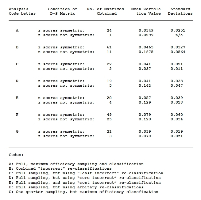
Table 1. See text for explanation.

     The results coded "Analysis A" reprise the results obtained and discussed in the last essay. Remembering that the random pattern simulation studies exposed considerably higher mean values from the correlation matrices derived from the initial spatial autocorrelation index matrices, the expectation here is that manipulations away from this standard (less dense sampling, inefficient classifications, etc.) should tend to produce higher figures than the .0349 average value reported here.

     "B" describes the outcome obtained from the manipulation described in #1 above--that is, when the numbers of points in each elevation class were exchanged for one another, creating inefficient classifications of the elevational variation (but again, not illogical ones: the effect was to shift the isolines separating classes of elevation, not to toss, for example, high and low elevations together). As can be seen, a larger proportion of the new derivations did not pass the symmetric double-standardized results test (11 of 72, to be exact); further, the average mean correlation value across all the 61 mean correlations of those that did, .0465, was in fact higher than the unmanipulated results.

     "C", "D" and "E" are used to label the breakdown of the manipulations discussed in #1 above into three groups (as described in #2 above), those most approximating the unmanipulated classifications, those ranking next, and those least approximating them. In Table 1, note that there is a slight trend toward fewer symmetric double-standardizations as approximation decreases, and also an increase in both the average mean correlation value and the accompanying standard deviations.

     "F" summarizes the analysis described in #3 above: namely, three arbitary re-settings per drainage basin of the elevation limits between classes of elevation in each, resulting in changes in the number of points connected with each class. The average mean correlation value across the systems that did attain symmetric double-standardized results is a now a considerably higher .079, as anticipated by the model; further, only about two-thirds of the systems (49) passed the basic test, a distant outcome compared to the 24 of 25 that did so in the unmanipulated tests.

     Lastly, "G" reports on the analyses run at one-quarter sampling density (as discussed in #4 above). Three of these did not pass the symmetry test, and those that did have, at .039, a slightly higher average mean correlation value connected to them.

     Thus, the manipulations discussed apparently did produce, to a fairly good approximation, the changes in results projected.

Results: Regression Analyses (#5 above)

     Table 2 summarizes the results of the follow-up regression studies discussed in #5 above.
 

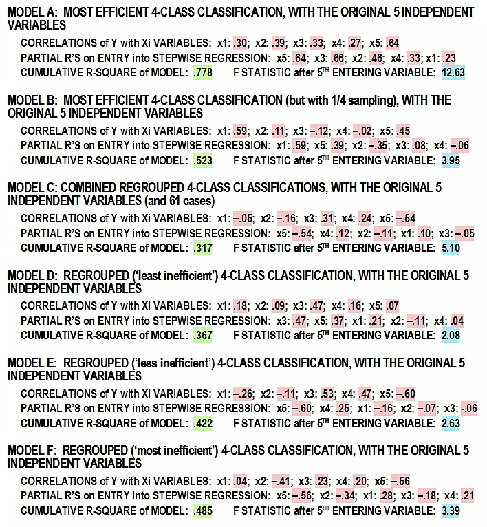
Table 2. See text for explanation.

     It will be recalled that the basic point of the follow-up multiple regression analyses was to investigate whether the degree of deviation from zero mean correlation conditions--that is to say, degree of system redundancy--could be predicted from independent variables describing levels of system disequilibrium, and measurement error. In this instance, disequilibrium represents lack of balance between erosional and depositional forces, and is manifest in topographical asymmetries connected to newly formed, rapidly changing, or geologically complex geographies. Importantly, one should expect on the basis of the model presented here that suboptimal classifications of the subsystem structure projected to exist will lead to dependent variable values whose prediction by the independent variables will only lead to weaker models.

     In Table 2 the first results presented, for Model A, summarize the stepwise prediction of the dependent variable--the mean correlation value connected with each of the initial twenty-five spatial autocorrelation matrices (i.e., one for each drainage basin)--by the five independent variables described in the table first presented in the last essay. Note three things: (1) the cumulative r-square of the model is a fairly substantial .778 (2) each of the independent variables correlates nontrivially with the dependent value (and importantly, with the right sign, positive), and (3) each variable enters into the regression equation with a partial r that is positive (again, as would be expected).

     It is not necessary to discuss in any detail the other five regression models, as it is apparent that all of them do an inferior job of accounting for the dependent variable, and on all counts just noted.

     A good number of additional, parallel, multiple regression models were created around the results of the 3-, 5-, and 6-class classification results. Inasmuch as these classifications are thought to represent statistical solutions only (i.e., the model suggests that they do not reflect latent structural relations within the actual systems), it was expected that none of these models would do as good, or even nearly as good, a job of secondarily explaining the average mean correlation values obtained--and they didn't.

Conclusion

     Not all of these secondary studies produced results that were dramatic, but overall they present a consistency of adherence to projected result that is difficult to resist. I expect that with denser sampling of the drainage basins, and with more perfectly worked out explanatory variables to aid in the construction of the regression models, even better comparative models should emerge. Nevertheless, for the moment, at least, I count these results as significant evidence in favor of the model presented here. Let us continue on to another context, this one at a rather larger scale.    

_________________________

Continue to Next Essay
Return to Writings Menu
Return to Home

Copyright 2006-2014 by Charles H. Smith. All rights reserved.
Materials from this site, whole or in part, may not be reposted or otherwise reproduced for publication without the written consent of Charles H. Smith.

Feedback: charles.smith@wku.edu
http://people.wku.edu/charles.smith/once/streams2.htm