[[p. 221]] The aspects of ecology to be considered regard primarily the study of the conditions under which groups of organisms exist. Such groups may be acted upon by their environment, and they may react upon it. If a set of properties in either system changes in such a way that the action of the first system on the second changes, this may cause changes in properties of the second system which alter the mode of action of the second system on the first. Circular causal paths can be established in this manner.

    It is well known from mathematical theory, and is abundantly illustrated by other contributions to this publication, that circular paths often exist which tend to be self-correcting within certain limits, but which break down, producing violent oscillations, when some variable in the system transgresses limiting values. When a breakdown of the self-correcting system takes place in nature, it may be expected to end in disaster for some element in the system which consequently disappears. The original system is thus destroyed, to be replaced by another in which the lost element plays no part. It is, therefore, usual to find in natural circular systems various mechanisms acting to damp oscillations, and self-correcting mechanisms may be introduced at several points in the circular path. The importance of such a multiple corrective system has already been made clear, particularly in Professor Wiener's contribution. The resulting stability, which appears to characterize most ecological systems, while it permits their persistence, makes investigation difficult.

    The systems to be described range from cases in which at least part of the self-regulatory mechanism depends on purely physical aspects of the structure of the earth, such as the disposition of oceans and continental masses, to cases where the self-regulatory mechanism depends on very elaborate behavior on the part of organisms or groups of organisms. No sharply defined categories can be recognized in this series. It is, however, convenient to establish a methodological division of the following kind.

    When a circular causal system involving a group of organisms is described in terms of the transfer of some substance through the system, without employing any purely biological enumeration, such as the size of a population, the mode of approach will be characterized as biogeochemical. When a circular causal system is described in terms of the variation in numbers of biological units or individuals, or, in other words, in terms of the variation in the sizes of populations, the mode of [[p. 222]] approach is characterized as biodemographic. In general, the biogeochemical approach is appropriate to the simpler cases which would ordinarily not be considered as involving teleological mechanisms, and the biodemographic to more complex cases, some of which might be regarded as involving teleological mechanisms.

THE BIOGEOCHEMICAL APPROACH

The Carbon Cycle in the Biosphere

    The Biological Cycle. In photosynthesis, green plants take up carbon dioxide from the atmosphere and hydrosphere and, using the energy of part of the solar spectrum, synthesize organic carbon compounds from the carbon dioxide. Part of the carbon dioxide is returned directly to the atmosphere in plant respiration. Most of the remaining organic carbon, produced photosynthetically, is returned indirectly either by the respiration of animals eating plants or by bacterial decomposition of dead plant or animal tissues. The qualitative aspect of this cycle is well known to every student of elementary biology. A quantitative statement is rarely attempted. The available quantitative information is summarized in the diagram of Figure 1, in which the rates of migration along the different paths are derived, from the works of Goldschmidt (1934), Noddack (1937), and of Riley (1944), supplemented by certain general considerations derived from the work of Lindeman (1941).

    It has been pointed out by Kostitzin (1935) that a cycle in which the rate of growth of consuming and decomposing organisms depends on the rate of photosynthetic production, and the latter depends on the rate of return of CO₂ to the atmosphere by decomposing and consuming organisms, would tend to oscillate according to Volterra's prey-predator equations. This oscillation would be accompanied by oscillations in the CO₂ content of the atmosphere. Rough estimates of the period of oscillation can be made from the available data included in Figure 1. It is evident from such computation that the period would be of the order of magnitude of months or years rather than of centuries.

    The problem of the constancy or variability of the carbon dioxide content of the atmosphere as a whole is a difficult one, owing to the large number of possible sources of purely local disturbance. The earlier data have been reviewed by Letts and Blake (1900) and, more recently, practically all the available information has been considered by Callendar (1940). It appears that the best series of nineteenth-century determinations, between 1866 and the end of the century, give mean values that vary very little, from 0.0287 to 0.0294 per cent. All series show variations dependent on meteorological and seasonal events, the highest mean content being in spring, 0.02971 per cent; the lowest, in summer, 0.02905 per cent. It is evident that any small variations due to inherent oscillations in the system would not be detected, but it is equally certain that

[[p. 223]]

Figure 1. The carbon cycle (quantities as cm.² × year^-1 ).

large oscillations, which might have effects on other systems, do not take place. During the twentieth century, there appears to have been a slight rise in the CO₂ of the air, at least in the northern hemisphere. The nature of this is discussed below.

    The Regulatory Effect of the Oceans. In considering changes in the CO₂ content of the atmosphere, it is important to remember that the quantity of the gas in the air, equivalent to 0.11 gm. C per cm² of earth's surface, is small compared to that in solution, mainly as carbonate and bicarbonate, in the ocean, equivalent to 5.5 gm. C per cm². Since the atmosphere and hydrosphere are in contact, the CaCO₃-Ca(HCO₃)₂-CO₂ system of the ocean acts as an enormous shock-absorber regulating the quantity of CO₂ in the air, as Schloesing (1880) pointed out long ago. This conclusion is usually accepted in the recent literature, though Callendar (1940) has supposed, on grounds that are critically examined [[p. 224]] below, that the regulatory mechanism of the ocean operates so slowly that it cannot cope with the additional burden of CO₂ produced by modern industry.

    It is desirable to consider the path by which carbon dioxide enters the ocean. While some exchange across the surface must occur, and rainwater presumably carries a small quantity of the gas directly to the sea, the major contribution undoubtedly is derived from river water. According to Conway's (1942) analysis of the great body of data collected by Clarke, the rivers of the world discharge 7.05 × 10¹⁴ gm. of CO₂ as carbonate, annually, into the ocean. While most of this carbonate is now derived from limestones, Clarke (1924) concluded that 8 per cent of the total quantity comes from the atmosphere. Actually, the atmospheric contribution to rivers, and so to the ocean, must be larger, because the data used are based on the residue after evaporation, i.e., on carbonate rather than bicarbonate. It is reasonably certain that the mean river water will contain more than twice the amount of CO₂ indicated by the carbonate content, for, not merely is it legitimate to assume that the bases are present as bicarbonate, but it also seems probable that there will be a slight excess of CO₂. Provisionally, therefore, it is probably safe to take 110 per cent of the observed value, or 7.7 × 10¹⁴ gm. CO₂, as representing the atmospheric contribution. At least the 7 × 10¹⁴ gm., or 120 CO₂ per cm² of earth's surface present in excess of the carbonate CO₂, must be returned annually to the atmosphere, as the alkaline earth carbonates are converted into globigerina ooze and other carbonate sediments. The action of the bicarbonate CO₂ of river water is therefore comparable to that of a conveyor belt, and the net direction of exchange across the surface of the ocean must be from the sea to the atmosphere. The available comparisons of the CO₂ tension of surface water and of the air with which it is in contact (Krogh, 1904; Buch, 1939 a & b) usually show a slight deficiency in the water, so that CO₂ would tend to pass from the atmosphere into the ocean. The determinations have, however, all been made in the North Atlantic or Arctic during the summer months. As Buch points out, in regions of upwelling and seasons of much vertical mixing the situation must be reversed, for the deeper water of the ocean is known to be in equilibrium with much more CO₂ than occurs in uncontaminated air. The overall excess of CO₂ brought into the ocean, and liberated by carbonate sedimentation, must be returned to the atmosphere by such upwelling and vertical mixing.

    Gains and Losses to the Cycle. Although the passage of carbon through the cyclical paths involving living matter and the ocean is the major event in the migration of the element, the cycle is not quite closed. Oxidized carbon is continually being lost to the lithosphere as carbonate sediments, and reduced carbon as dispersed organic carbon in shales, as well as in coal and oil, though these concentrates are quantitatively insignificant in the present context. The total quantity of fossil carbon in [[p. 225]] the sediments is difficult to determine. For the carbonate sediments, Goldschmidt (1934) gives 6600 gm. CO₂ per cm² or 1800 gm. C per cm²; Noddack (1937) gives 8000 gm. CO₂ per cm² or 2200 gm. C per cm². The higher of these values, which are at any rate fairly concordant, will be used for reasons that will appear below.

    The mean concentration of organic or reduced carbon in the sediments is taken by Goldschmidt to be about 0.2 per cent. This figure seems to be based not only on the available analyses but on certain considerations relating to the oxygen balance of the biosphere. Noddack gives a much higher weighted mean, namely 0.76 per cent C. This is based on an estimate of 0.94 per cent C in shales, for which no analytical evidence is available. The best analyses for shales (Clarke, 1904) give a mean of 0.81 per cent C, and taking the shales as constituting 80 per cent of the sediments, the weighted mean is 0.66 per cent, which in a column of sediment of 170 kg. per cm² corresponds to about 1100 gm. per cm². The following considerations (Kamen, 1946) indicate that such a value is of the correct order of magnitude.

    Carbonate precipitated from aqueous solution in contact with atmospheric CO₂ is slightly enriched in C¹³ over the carbon of plutonic rocks. The carbon that remains after carbonate has been precipitated is, in consequence, slightly impoverished in the heavy isotope.

    In a series of determinations of the isotopic ratio, Nier and Gulbransen (1939) found the mean value of C¹²:C¹³ for primary carbon (diamond, graphite, meteoritic) to be 89.4. Three limestones of varying age gave 88.3, specimens of recent and fossil plant carbon 91.4. These results suggest that in the course of geological time about twice as much carbonate carbon as reduced carbon has been deposited in the sediments. A later study by Murphey and Nier (1941) confirms the difference between plant carbon and carbonate carbon, and indicates no difference between fossil and recent specimens. The results of the later study apparently cannot be used with the earlier investigation, because, although the differences between the ratios within each series are reasonably accurate, the absolute values are apparently subject to instrumental error. In the second series, the primary carbon samples are overweighted in favor of meteorites, only one terrestrial specimen being examined, so that it is difficult to know what value to use for the original material from which the carbon of plants and limestones came. Accepting provisionally the results of the first series, it is clear that they are in good accord with the geochemical estimate of 2200 gm. per cm² carbonate carbon and 1100 gm. per cm² organic carbon. Accepting a 2:1 ratio, if Goldschmidt's value of 1800 gm. of carbonate carbon per cm. be more accurate than Noddack's, the corresponding reduced carbon would be 900 gm. per cm², corresponding to 0.53 per cent C in the mean sediment. The reason for Goldschmidt's conclusion that the reduced carbon content of the sediments is considerably lower than even this estimate, appears to lie in his consideration of the oxygen content of the sediments. During the [[p. 226]] process of erosion and sedimentation, oxidation of the sediments takes place. The oxygen lost in such a process may be assumed to be of photosynthetic origin. An equivalent quantity of reduced carbon should therefore be fossilized. Goldschmidt finds that the maximum possible amount of fossil oxygen corresponds to but 0.17 per cent reduced carbon in the sediments, and this figure has clearly influenced his estimate. Actually, it seems inevitable to accept the lack of balance implied by the excess of reduced carbon in the sediments which presumably can be explained (Poole, 1941; Conway, 1943; Cotton, 1944) by the oxidation of methane, carbon monoxide, hydrogen, and sulphur dioxide in volcano gases.

    The 2200 gm. per cm² of carbonate carbon and 1100 gm. per cm² of organic carbon correspond to 12,100 gm. of CO₂ per cm² of the earth's surface. In other words, since the beginning of sedimentation, approximately twelve atmospheres of CO₂ have been removed from the biosphere. The available evidence strongly suggests (Conway, 1943) that this immense quantity of CO₂ did not exist all at one time in the atmosphere, but has been added and removed gradually. It has long been realized that volcano gases supply the required source of carbon dioxide. No direct measurements of the output of the gas from volcanos are as yet available. The only estimate for the rate of production of volcanic CO₂ that can now be made is obtained by dividing the carbon lost to the sediments by the geological time-span of 1.5 × 10⁹ years. The result is 8.0 CO₂ or 2.2 C per cm² per year. Goldschmidt used a rather lower figure (3-6 CO₂ per cm² per year) for reasons that are already apparent. It has been pointed out before that 7.7 × 10¹⁴ gm. CO₂ or 132 per cm² are apparently brought into the sea, annually, by rivers. Most of this CO₂ is evidently returned to the air, but Clarke concluded that 8 per cent of the CO₂ of carbonates is of atmospheric origin. These 8 per cent or 10 per cm² per year will be lost to the cycle and should be of the same order of magnitude as the 8.0 CO₂ which are known to be fossilized as carbonate, or after reduction. In view of the uncertainties involved, the agreement is highly satisfactory.¹

    The Efficacy of Self-Regulatory Mechanisms. Callendar (1940), considering the best data available since 1866, concludes that during the present century there has been an increase of the order of 10 per cent in the CO₂ content of the atmosphere. This he attributes to the modern industrial combustion of fuel. He points out that if the increase in CO₂ content observed is uniform throughout the atmosphere, it corresponds to an accession of 2 × 10¹⁰ tons. The total addition during the period 1900-1935 from fossil fuel is taken as equivalent to 1.5 × 10¹⁰ tons of CO₂. In view of the difficulties in obtaining good representative series [[p. 227]] of data on CO₂, the agreement would appear to be satisfactory. Callendar supposes that the regulatory mechanism of the ocean operates so slowly than an increase in CO₂ at the rate implied cannot be controlled and that the whole of the industrial CO₂ output of the first third of the twentieth century has remained in the atmosphere. There are, however, two very grave objections to accepting this conclusion.

    The rate of industrial production of CO₂ used by Callendar is 4.3 × 10⁸ tons per year, or essentially the same as that implied in Goldschmidt's estimate of 800 per cm² per year. The corresponding value in terms of carbon is 1.2 × 10⁸ tons. Riley's most probable estimate of the total rate of photosynthetic fixation, and consequently of liberation of CO₂ by respiration and fermentation, is 1460 × 10⁸ tons, while for terrestrial areas Noddack's value is 151 × 10⁸ tons. The rate of industrial production is therefore of the order of 1 per cent of the rate of biological production on land and of 0.1 per cent of the rate for the whole earth. Assuming the validity of Callendar's conclusion that transport through the sea surface is not involved, it is apparent that for his view to be correct it is necessary also to suppose that the mechanism of the biosphere is such that a very accurate regulation occurred during the nineteenth century, but that during the twentieth an increase of the order of 1 per cent in the total production of CO₂ was quantitatively rejected by the system. This is extremely improbable.

    In addition to this theoretical difficulty, there exist observational data of great significance. Glückauf (1944) has determined the CO₂ content of twelve samples of air taken from altitudes of 4,000 to 10,000 meters over Great Britain. His results range from 0.024 to 0.030, the mean being 0.025±0.001 per cent, which is slightly lower than the mean of the lowest series of nineteenth-century determinations. Analyses of air at ground level by the same technique as was used in the analysis of the upper-air samples gave values of 0.031-0.035 per cent in accord with other modern determinations. If Callendar's hypothesis be adopted, it is necessary to reject any free interchange of air above 4,000 meters since late Victorian times, which is absurd.

    The true interpretation of these results would appear to be a slight change in the distribution of stationary concentrations of CO₂ passing through the system, rather than a static accumulation of the gas. Since the upper-air values are lower than those at ground level, and since there is no obvious way for CO₂ to be lost in the upper troposphere, a full elucidation of the problem must await determinations of the origin of the air masses in question. There must be sinks as well as sources in the atmospheric circulation of the gas. If, as seems probable, the sinks are local areas of ocean surface, they have not yet been discovered on a scale commensurate with what is required. Meanwhile, it seems far more likely that the observed increment in the carbon dioxide of air at low levels in both Europe and eastern North America is due to changes in the biological mechanisms of the cycle rather than to an increase in industrial [[p. 228]] output. It is quite probable that the net effect of the spread of the technological cultures of the North Atlantic basin has been to decrease the photosynthetic efficiency of the land surfaces of the earth. Though the most productive agricultural land, on which corn is cultivated, can have a photosynthetic efficiency greater than that of the best temperate forest, it is very unlikely that, in general, cleared farm land is as biologically productive as is virgin forest. Moreover, it is obvious that long-term readjustments, due to increasing photosynthesis with increasing CO₂ pressure over a period of years, are less likely to be effective on agricultural land because the biological community is annually built up again from nothing, while gains of one year in tree growth are likely to be reflected as increased photosynthetic surface in the succeeding year. The hypothesis that deforestation, perhaps coupled with soil erosion and loss of nutrients to the sea, has changed the composition of the atmosphere over the land during this century at least demands serious consideration. Whatever the ultimate solution of this problem may be, Glückauf's results certainly indicate that the self-regulating mechanisms of the carbon cycle can cope with the present influx of carbon of fossil origin, even though changes in the pattern of steady-state concentrations may have occurred.

    A further aspect of this problem must be briefly considered. If the conclusion that has just been reached is correct, it is apparent that the addition of CO₂ at a rate corresponding to a hundred-fold increase in vulcanism is not sufficient to derange the main self-regulatory processes. There is, therefore, little likelihood that a moderate decrease or increase in vulcanism during the past has had any significant effect on the overall regulation of the CO₂ content of the atmosphere. Moreover, if the modern increase is correctly ascribed to human interference with the biological mechanism of regulation, it is improbable that changes in vulcanism per se could have produced significant changes in the pattern of steady-state concentrations. It is, however, reasonable to suppose that changes in the emergence of the continents may have had some small effects by altering the area of the terrestrial plant cover, while greater effects may be reasonably attributed to the major evolutionary steps in the development of the land flora.

    A Possible Change in the Productivity of the Ocean. The only hint of any change in the quantitative aspects of the carbon cycle that can be derived from the geological record suggests that the Palaeozoic sea was slightly more productive than the Mesozoic or Tertiary ocean. Clarke (1904) gives the mean carbon content of fifty-one Palaeozoic shales as 0.88 per cent, while that of 27 Mesozoic and Cenozoic shales was found to be 0.69 per cent. The significance of such a difference is increased by the finding of Miller (1903; Hall and Miller, 1908) of a mean content of 0.65 per cent C in a collection of shales and clays, mainly Mesozoic, from Britain. If subsequent analyses confirm the slightly greater carbon [[p. 229]] content in the older shales, it will be apparent that more organic carbon per gram of argillaceous matter was deposited in the Palaeozoic than at a later date.

    The Methane Cycle. An alternative path, involving the liberation of methane to the atmosphere, is seldom considered. Though this process is much less impressive than that of the return of carbon to the air as CO₂, there clearly must be a mechanism for removal of methane, if it is not to accumulate. The data implying the existence of a minor but nevertheless significant methane cycle are derived from a consideration of the gaseous exchanges of large herbivores. Benedict and his co-workers have shown that fermentation in the alimentary canal of such animals gives rise to so much methane that a significant proportion of the carbon of the food ingested is lost in the expired air as CH₄. Table 1, which follows, has been prepared by Mrs. Jane K. Setlow, using the data for the world populations of domestic animals collected by Rew (1928) and those for production per day per animal given by Ritzman and Benedict (1938).

    The total production is probably considerably greater than the sum given in Table 1. Not only must an extensive but unknown population of large ungulates, notably antelopes, various species of wild Bovinae, and deer be considered, but also the large production of methane in swamps and lakes for which no satisfactory estimate is possible at present. It is probably quite safe to double the estimate given in the table, and not unlikely that the resulting figure of about ninety million metric tons is too low. Such a quantity corresponds to about 0.06 per cent of the annual photosynthetic fixation of carbon. It is obvious that unless mechanisms for the oxidation of methane exist, circulating carbon would slowly accumulate in the atmosphere. Three possible methods of oxidation appear to exist:

(1) A small amount of direct combustion in lighting flasks and on hot lava surfaces may be expected.
(2) Photochemical oxidation might be expected in the stratosphere.
(3) Bacterial oxidation certainly occurs in soils.

The second and third mechanisms seem more likely to be important than the first, though both of them take place in regions more or less cut off [[p. 230]] from the turbulent diffusion of the troposphere. It would, indeed, appear remarkable that the suggested mechanisms of oxidation are sufficient to keep the stationary concentration of methane in the atmosphere at an almost undetectably low level (Hutchinson, in press).²

    General Properties of the Carbon Cycle. It will be apparent that two main self-corrective systems exist in the carbon cycle, namely, the CO₂-bicarbonate-carbonate system involving air, sea, and sediments, and the biological photosynthetic cycle. The first of these involves a reversible chemical equilibrium, the rate of establishment of which is in part determined by physiographic factors, while the second involves an irreversible path which could theoretically give rise to oscillations but which probably does not do so because of the damping action of the first mechanism. The distribution of steady-state concentrations in the atmosphere probably depends on both mechanisms. It has undoubtedly altered in the past half-century, probably owing to changes in the vegetation cover of the earth. An alternative path in the carbon cycle, involving methane, certainly exists, though it is not likely to be of significance in determining the self-regulatory properties of the whole cycle.

    Several other biogeochemical cycles involving passage through the atmosphere exist. By far the most important of these is the nitrogen cycle. In the cycles of sulfur and of the halogens, transport through the atmosphere also undoubtedly plays a part, but the quantitative details are little known. The nitrogen cycle is far more complicated than that of carbon. In the carbon cycle, the only important compounds circulating freely outside organisms are CO₂ and carbonates among the oxidized carbon compounds, and methane among the reduced carbon compounds. In the nitrogen cycle, ammonia, molecular nitrogen, and several oxides are certainly present in the atmosphere, though the stationary concentrations of all but N₂ are minute. Ammonia, nitrate, and often nitrite are present in the hydrosphere. Several alternative paths exist in the cycle. Cooper (1937) gives a good modern presentation. Quantitative biogeochemical data are, however, very inadequate. Most of the information that exists has been considered in an earlier paper (Hutchinson, 1944a). It is reasonably certain that both fixation of N₂ and formation of N₂ from nitrogen compounds are mainly mediated biologically. It is also obvious that the steady-state position relative to fixation and formation of molecular nitrogen is such that nearly all the nitrogen is in the molecular condition. There is, moreover, adequate evidence that the fixation process is highly inefficient and consumes a significant fraction, conceivably of the order of n × 10 per cent of the total energy fixed photosynthetically. The nitrogen cycle is thus linked to the carbon cycle. The linkage, moreover, involves circular paths, for not only is the total rate of entry of molecular nitrogen into biological systems likely [[p. 231]] to depend on the rate of photosynthesis, but the rate of photosynthesis is, clearly, in part determined by the steady-state concentration of nitrogen compounds available for the maintenance of plant populations. It is evident, too, that both cycles in part depend on the rate of liberation of phosphorus from the lithosphere on land and the rate of regeneration of phosphorus by vertical mixing in the sea. Thus, it is possible that the biological cycle of the elements must be regarded as a unity, the rate of working of which is primarily determined by non-biological factors, such as precipitation, winds, currents, and the disposition of the continents and oceans.

The Phosphorus Cycle in Inland Lakes

    Biological Productivity and Phosphorus Concentration. The second biogeochemical example to be discussed relates to much smaller systems than the entire biosphere. Such systems, being much younger than the biosphere, throw light on the mechanisms by which a steady state in the cycle is achieved.

    In a series of small inland lakes of similar area and depth, there is evidence that the variation in the total quantity of living matter inhabiting the water and the mud depends primarily on the supply of phosphate and combined nitrogen that can pass from the drainage basin into the lake. All other nutrient elements are likely to be present in excess in inland waters. If a colorless bottle of lake water is suspended at the surface of the lake from a buoy, little change in the total quantity of phytoplankton in the bottle will occur in the course of a week. Addition of a small quantity of phosphate and nitrate, however, will in a similar span of time cause a great increase in the total quantity of plant material in the water enclosed in the bottle. Since no appreciable amounts of phosphorus enter the atmosphere, and since the phosphorus cycle rarely involves any compounds less oxidized than phosphate, this cycle presents simpler features than does that of nitrogen. The phosphorus cycle will therefore be used to provide the main basis for the argument, though in general a parallel movement of nitrogen compounds can be assumed.

    At least during the summer months, the planktonic algae keep the concentration of phosphate at a hardly traceable low level, rarely in excess of a few micrograms per liter. The algal cells, most of which probably require 10 per liter phosphate phosphorus for optimal growth, are evidently living in a state of chronic starvation, and any small addition to the nutrient salts of the water is presumably taken up rapidly. At the same time, algal cells are being eaten by animals; some part of the algal material is constantly being incorporated into fecal pellets, and these, being larger than the algae, sediment more rapidly.³ This rain of feces must constitute a drain on the phosphorus supply of the illuminated [[p. 232]] upper water of the lake. Moreover, changing conditions of temperature and perhaps of illumination lead, directly or indirectly, to changes in the specific composition of the microscopic algal flora, so that populations of algae are continually dying and sinking. Animal deaths again must remove material in the same way. There is, thus, a continual falling of material from the illuminated water to the bottom of the lake, and this falling must remove the various constituents of living matter, among which phosphorus is notable. In shallow lakes, regeneration of the phosphorus can occur through the wind-generated circulation of the water, which will bring material that is diffusing from the mud into the illuminated layers where phytoplankton can grow. In deep lakes, the illuminated trophogenic waters tend to be cut off from the lower layers, which remain cold throughout the summer. A great deal of indirect evidence (Hutchinson, 1941) shows that enough horizontal movement of water occurs at all depths, even in very stably stratified lakes, to bring phosphorus from the mud into the open water. In a lake in which practically no vertical mixing of water is occurring except in the top meter or two, the phytoplankton is continually growing and sedimenting, thus removing phosphorus from the illuminated zone, and this phosphorus is continually being replaced, by movement of phosphate liberated by decomposition, from the mud into the open water. It has recently been possible to confirm the existence of this cycle by the use of radiophosphorus (Hutchinson and Bowen, 1947, in press).⁴

    The factors controlling the rates of the various parts of this cyclical migration are practically unanalyzed and are certainly very complex. Physical events external to the cycle possibly play a preponderant role and may prevent the recognition of any clear self-regulatory mechanisms when the process is studied over a short time-span. An indirect approach to the study of the problem over long periods of time is, however, possible.

    The Growth of the System. The nutrient cycle in a lake is not quite closed. Small quantities of nutrient elements are being brought into the lake by the inlets and by the seepage of ground water. Small amounts are, likewise, lost through the outlets and to the sediments deposited on the lake bottom. At least in biologically productive lakes, the rates of such gains and losses are very small, compared to the rate of transfer through the cycle. Their existence, however, makes further analysis possible. When a steady state is achieved, the losses will just balance the gains, and part of the losses are available to analysis through the study of sediment profiles collected with various boring devices.

    [[p. 233]] If a lake sediment be poor in organic matter, little regeneration of nutrient substances will take place from it. There will be little organic nitrogen present to produce ammonia or nitrate, and though some phosphorus will probably be present in the inorganic fraction, it will be in the form of insoluble minerals. A little of such phosphorus can go into solution and support algal growth, as Strøm has shown in the case of the inorganic silts of Norwegian mountain lakes, but the rate of liberation of phosphate from such a deposit is likely to be very slow. If, however, the sediment be rich in organic matter, there will be much nitrogen to pass into solution as the result of bacterial metabolism, the phosphorus of organic origin will usually be freely soluble, and the carbon dioxide present in the mud may facilitate the solution of the mineral phosphates.

    In temperate regions, where decomposition on the lake bottom is slow, the condition for the presence of primarily inorganic sediments is that little organic material be produced in the lake, the condition for the existence of a richly organic sediment being the production of much organic matter in the lake. Some additions from the vegetation of the catchment basin may be expected in all cases, but it appears that such additions do not alter the character of the process to be described.

    Starting with a barren glacial basin newly filled with water, the concentration of phosphate in solution in the drainage basin will depend on the general geochemistry of the region. At first, the nitrogen available will probably be derived solely from rain water, but nitrogen will tend to be fixed biologically, according to the availability of organic matter, the production of which will depend on the availability of phosphorus and other mineral nutrients. The water of the lake will gradually develop a phytoplankton population. The first sediments to be deposited will be almost entirely inorganic, but as soon as remains of organisms are included in the surface layer of these sediments, an internal cycle of the kind already described will be established. Phosphate will be more easily liberated from mineral particles, owing to the production of carbon dioxide by decomposition, and the phosphate of the decomposing organisms will be returned to the lake water. As productivity increases, the sediments will become more and more organic, and thus more and more able to return the nutrients rapidly to the cycle. This process continues until the geochemically determined nutrient potential of the silt and the water of the drainage basin is fully utilized. In a eutrophic region, rich in nutrients, the final result will be a fertile lake, while in an oligotrophic region, poor in nutrients, it will be a relatively sterile lake (Figure 2).

    The general interpretation just given was derived from a study of the sedimentary cores collected by Dr. E. S. Deevey in Linsley Pond, a small, rather productive lake in North Branford, Connecticut (Hutchinson and Wollack, 1940). It was apparent from a study of these sediments that initially the productivity of the lake was very low, but that it then rose with increasing rapidity. Later, the rise in productivity was checked, [[p. 234]] and a long period set in during which some irregular variations, but no great divergence from an essentially constant steady-state condition

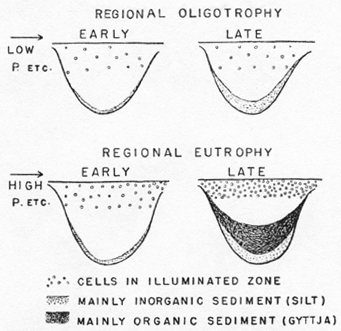
Figure 2. Ideal diagram of early and late stages in the development of a lake in an oligotrophic or nutrient-poor region, and in a eutrophic or nutrient-rich region.

occurred (Figure 3). This steady-state condition was evidently terminated by settlement in the eighteenth century, accompanied by deforestation, soil erosion, and rapid, complex changes in the lake. Subsequent to our studies, Pennington (1943; Jenkin, Mortimer, and Pennington, 1941) has obtained evidence of the same type of development in Windermere, in the English Lake District. In Pennington's profiles, the steady state is much more regularly maintained than in Linsley Pond, no doubt owing to the much greater size of Windermere and the consequent stability of the biological community in the face of external disturbances such as drought or forest fires. Pennington adopted an absolute time scale based on sedimentation rate within the lake, and this scale has been confirmed by Pearsall's (1946) recognition of two levels of increase in grass pollen as corresponding to Neolithic settlement about 1100 B.C. and Norse settlement between 1200 and 1400 A.D. Extrapolation beyond the verified part of the time scale gives the duration of the steady-state period as about 6000 years. Eastern North American pollen profiles cannot yet be referred to an absolute [[p. 235]] chronology, but there can be little doubt that the steady-state period in Linsley Pond lasted several thousand years, too.

Figure 3. Ignitable matter, lignin and crude protein per gram of inorganic matter, as measures of organic production, plotted against total accumulation of inorganic sediment, as a measure of time. The final decline in all three curves is undoubtedly due to silt brought in at an abnormal rate after clearance and cultivation of the lake basin.

    The steady-state period is recognized by the essential constancy in composition of its sediments. This is taken to mean that the productivity of the lake per unit area does not vary. Meanwhile, the lake is filling up with sediment, and the volume is therefore diminishing. Any properties of the lake dependent on the ratio of productivity to volume will, consequently, change. The volume of deep water cut off from circulation during the summer months will decrease, but not the organic matter that falls into it. The oxygen lost in a summer from unit volume of such water will therefore increase, and this progressive change will greatly change the qualitative aspects of the fauna. From a study of the arthropod remains fossilized in the mud, Deevey (1942) has beautifully shown how this happened in Linsley Pond. To the taxonomic biologist, the lake [[p. 236]] early in the steady-state period would have seemed an entirely different locality from the lake at a late stage.

    If the organic matter of the sediments may be used as a measure of productivity, it appears, therefore, that the variation of productivity with time can be expressed by a curve not unlike the sigmoid curve of growth, but that once the nutrient potential is being used with maximum efficiency, a number of purely qualitative changes can take place without altering the overall quantitative picture. The general mechanism of the steady state is comparable to the large self-regulatory cycles of the biosphere, the growth of the system being comparable to the growth of homogeneous populations to be discussed below. It is tempting to speculate as to whether, originally, living matter did not increase according to a like sigmoid law. After such a rapid expansion, vast qualitative changes with little quantitative variation in the total size of the system may have taken place.

THE BIODEMOGRAPHIC APPROACH

Unlimited and Restricted Growth

    The unrestricted growth of a population, N, with a zero death-rate, such as a protozoan or bacterial culture dividing under constant environmental conditions, will be represented by the differential equation

dN / dt = Nb,

where b is the reproductive rate. For higher metazoa, the same law would be obeyed, if we regard b as the effective reproductive rate or difference between birth- and death-rate. In practice, some limit is obviously always imposed on this Malthusian expansion. It is usually assumed that the effect of the limiting conditions will tend to operate feebly but with an increasing effectiveness from the beginning of the expansion. The simplest expression of this situation is obtained by supposing b to be multiplied by a factor which measures the proportion of space still remaining for the population to occupy. If the saturation value be K, then

(dN / dt) = Nb ((K-N) / K).

This is the derivative of the familiar Verhulst-Pearl logistic or sigmoid curve of growth. It is usually closely approximated in the growth of experimental populations that can be maintained under constant conditions, and for the study of such populations the use of the equation is fully justified in practice, even though it is hardly possible, in most cases, to decide between the logistic and certain other more complex expressions that have been proposed.

    The Verhulst-Pearl logistic is not only applicable to populations. It [[p. 237]] describes the growth of many single organisms or their parts. It is usual to regard organisms and their parts as growing like populations of protozoa or bacteria, by cell division. This, however, is clearly not necessary in order to produce a growth curve of the sigmoid form implied by the logistic, because in many cases most of the cell division occurs early in the process, while the later stages of growth occur solely through increase in cell size.

    It has been indicated in the previous section of the paper that a qualitatively similar growth curve applies to the whole biocoenosis of a lake. In this case, we have no necessary organic continuity between the organisms of the biocoenosis early and late in the process. As has been indicated in detail, early colonizations insure that the geochemically determined trophic potential is used with increasing efficiency by later organisms, until a maximum efficiency is reached. It will be obvious that this represents a process formally analogous to, though biologically distinct from, the reproduction of the members of a population increasing towards a maximum defined by the trophic potential. The same analogy, but a different distinction in mechanism, is implied when sigmoid growth curves occur in economics (Lotka, 1925).

    It is legitimate to regard the term K-N / K as formally describing a self-regulatory mechanism. There can be little doubt that, biologically, the mechanism can take a great variety of forms. The only formal condition that must be imposed on the biologically possible mechanisms is that they operate so rapidly that the lag, T, is negligible between t when any given value of N is reached, and the establishment of the appropriately corrected value of the effective reproductive rate b (K-N / K).

    If there is a time lag such that the rate dN / dt at time t is determined by N_(t-), then oscillations will be introduced into the system. The growth curve will pass the saturation level K at, e.g., t₁, and then at time t_l + the rate of change of the population will become zero. The population will then decline, reaching K, now from above, at t₂, and again at t₂ + the rate will become zero and the curve will then approach K from below. Further work is needed in the analysis of this case,⁵ but it is evident that the longer T, the more will N surpass the saturation value in the first ascent of the curve. For small values T, the oscillations will die out and the saturation value will be approached.

    [[p. 238]] It is quite likely that a number of cases of this phenomenon will be discovered. Pratt (1943) has shown that, in Daphnia populations, oscillations can be set up which are in part due to the fact that the fertility of a parthenogenetic female is determined not merely by the population density at a given time but also by the past densities to which it has been exposed. Much recent work on rodent populations reviewed by Elton (1942) and by Errington (1946) indicates that at high densities a great deal of intraspecific fighting may take place. Younger animals about to embark on their reproductive career are more likely to succumb in such fighting than are old experienced animals whose remaining reproductive career is short. The net result of fighting at high density is to change the age composition of the population in favor of old non-reproductive individuals, which soon die off from other causes. In nature, the events are not continuous, but dependent on a seasonal cycle which probably enhances oscillations generated by the purely internal demographic factors. It is quite possible that phenomena of this sort, which, in effect, involve the operation, with a time lag, of population density on net rate of increase, play a part in generating the well-known cyclic changes in the populations of field mice. Though it is probable that many more cases of the operation of time lags could be found, it seems likely, from the number of certain cases where they do not operate, that the phenomenon is relatively rare. It is highly probable that there is a general tendency for the time lag to be reduced as much as possible by natural selection. Supersaturated values of the population may introduce new unfavorable conditions, causing epidemics or other disasters, while if this does not happen the population is likely to be exposed to greater risk of extermination by chance unfavorable factors at the times of the subsequent minima in the oscillation. In spite of some glaring exceptions, it seems probable that an internally oscillating population is less likely to survive indefinitely than a stable one. If this be so, the time lags will be reduced to minimal values.

    Competition and the Balance of Nature. Volterra (1926) and Gause (1934-1935) have examined what happens when two populations are competing for a food supply maintained at a constant level

where a and  are coefficients of competition, indicating the depressive effect of a unit of one population on a unit of the other. Negative values of both a and correspond to symbiosis, a positive value of one and a negative value of the other to certain kinds of commensalism and parasitism (Gause and Witt, 1935). When mutual competition takes place, both coefficients being positive, three cases may be distinguished:

[[p. 239]]

(1)

    The members of each species act unfavorably on the members of the other, more powerfully than they do on the members of their own species. The final result is that only one species is left, and the species to survive is determined by the initial proportion. Gause had no example of this phenomenon, but it could probably be realized in cultures of microorganisms producing mutually inhibitory antibiotics.

(2)

    Competition takes place, and the final result, whatever the initial condition, is determined by the relative values of the coefficients. This case has been generalized for n species by Volterra.

(3)

    Both species survive indefinitely at an equilibrium concentration.

    When competition for food is involved, it is obvious that (3) can be realized if a system be set up in which competition could lead to displacement of species 1 by species 2 and at the same time a volume of space, termed a refuge by Gause, be provided into which species 2 cannot go. More generally, if there are two spatially defined regions, in one of which a > (K₁ / K₂), < (K₂ / K₁) and in the other a < (K₁ / K₂), > (K₂ / K₁), then the conditions of (3) can be realized and the species can coexist. Following the usual terminology, the two species are said to have separate though partly overlapping niches, and so long as this is the case they can persist indefinitely. In general, wherever in nature two species coexist in a region and feed on the same food, they will be found to have slightly different ranges of environmental requirements. It is commonly recognized by ecologists that closely allied species living together practically always occupy slightly different niches or, in other words, have different tolerances and optima. Two possible exceptions to this rule may be expected. (1) Where some external factor acts to rarify the mixed population, so that the environment possibilities are hardly exploited, the process of expulsion of one species by the other might never progress beyond the initial stages (cf. Crombie, 1945). A powerful and quite indiscriminate predator might maintain two species of prey at such a low level that they never come into effective competition. (2) Where the values of a and are under environmental control, as is indeed implied by the theory of niches, continual chance oscillations of the environmental variables might continually reverse the direction of competition, so that no equilibrium could ever be established. The numbers of the competition vary [[p. 240]] irregularly, but all are always present. It has been suggested that this situation is exemplified by mixed phytoplankton populations in lakes (Hutchinson, 1944b).

    Prey-Predator Relationships. The most striking theoretical results involving biodemographic circular causality are probably those of Lotka (1925), Volterra (1926), and other investigators on prey-predator and host-parasite relationships. The simplest case, considered by Volterra, may be developed as follows:

    If N₁ be the number of prey and N₂ the number of predators, and predation is taken to be proportional to the number of random encounters, then, if the populations are sufficiently sparse to permit neglecting the regulatory mechanism discussed in the previous section,

where b₁ is the effective birth-rate of the prey in the absence of predation, d₂ the effective death-rate of predator in the absence of food, and p₁ and p₂ coefficients expressing the effect of predation on the two populations. The solution of this pair of simultaneous differential equations is

which, when N₁ is plotted against N₂, gives a series of closed curves moving round the singular point

N₁ = (d₂ / p₂), N₂ = (b₁ / p₁)

It is important to note that p₂, the efficiency with which individuals of prey are converted into predator, depends on p₁, the efficiency with which predators kill prey. It is probably not unreasonable to write kp₁ for p₂. Thus, the greater the likelihood that death of prey follows encounters, the closer the singular point is to the origin. Gause has found experimentally that if the predation rate be maintained artificially low by continual rarification of the predators, then the cyclical variation postulated by Volterra does take place, but that in a confined system with predatory microorganisms feeding at their natural rate, the values of the predation coefficients are so great that oscillation around the singular point becomes statistically impossible. In other cases, other, more complex, situations, which in effect raise the predation rate, may develop. In nature, the only cases where it seems likely that typical Lotka-Volterra oscillations develop is where organisms live in a rather dense medium, such as soil or flour, which impedes free movement. The [[p. 241]] classical cases of persistent oscillations, such as the snowshoe rabbit, Lepus americanus, and the lynx, Lynx canadensis, are unlikely to be due to the prey-predator relationship, because they seem to occur in a prey population in the absence of the predator.

    The Classification of Periodicities in Populations. Some of the material that has been presented above may provide a useful scheme for the clarification of cyclical phenomena in populations. It is desirable, first, to point out that in a great many cases of fluctuation in animal populations where periodicities have allegedly been detected, they are probably of a spurious nature.

    If some environmental variable, x, fluctuates over a range of values, and p is the probability of values in excess of a certain given value, k, and if the occurrence of a certain biological event be implied by the condition x is greater than or equal to k, then it is clear that p is the probability of the occurrence of the biological event. Now if p be taken as constant over a long time-span and if two parts of the time-span be compared, the frequency of occurrence of the biological event will be approximately the same in the two parts of the time-span. If, in such a case, the biological system has an autoregressive property, so that its state depends on all previous states, as well as on the value of x at the time under consideration, the variation of the biological system will be smoothed, often showing quasi-periodic movements of low persistence, and also occasional great irregular increases or decreases reminiscent of the irregularly occurring years of excessive abundance or scarcity so often encountered in nature.⁶ It seems not unlikely that the supposed cycles with a 5- to 6-year period in British game animals described by Middleton (1934) are, in part, of this nature.

    Rejecting the statistical quasi-periodicities of this sort, we may, theoretically, distinguish cases in which the periodicity is extrinsic from those in which it is intrinsic. The valid cases of extrinsic periodicities are mainly determined by diurnal, lunar, tidal, or annual periods; in other words, by the mechanical properties of the solar system. There can be little doubt that there often are solar rhythms corresponding to the sunspot cycles observable in tree growth, but the evidence that such rhythms are reflected in the variations of animal populations is totally inadequate. A few cases in which fairly regular extrinsic periodicities are imposed on populations by periodic meteorological phenomena have been described. The best case is probably the variation of the population of the guanay Phalacrocorax bougainvillei on the Peruvian coast in response to abnormal hydrography, seemingly with a period of about seven years. This case will be critically discussed in detail in a later publication.

    [[p. 242]] Intrinsic periodicities are presumably best divided into cases in which the factors producing a decline are operative throughout the cycle, as in the case of predation, or those in which they only operate at abnormal densities, as in pandemic disease. Where the operation is continuous, there is an obvious dichotomy between the interaction of a population with itself at a later time and the interaction of two populations of different species. Finally, there are cases in which the periodicity is intrinsic to one species but entirely extrinsic to others. The classification may be expressed as follows:

I. Extrinsic to biological community.
    (a) Planetary mechanical, e.g., diurnal, tidal, lunar, or annual.
    (b) Solar (very doubtful).
    (c) Other meteorologically determined cycles.

II. Intrinsic to biological community.
    (a) Mechanism of decline discontinuous.
    (b) Mechanism of decline continuous;
        (1) Interaction within a species,
        (2) Interaction of more than one species.
    (c) Derived periodicity extrinsic to species under consideration, intrinsic to
         another species.

    Oscillation and Natural Selection. The theoretical approach to circular causal systems in ecology suggests that these oscillating systems should be found frequently in nature. Certain oscillations have been discovered and have been investigated extensively, though little understanding of their nature has been achieved. Practically no cases can as yet be placed in their proper categories in the theoretical scheme. The great attention that has been paid to the few good examples, notable to the periodicity of microtine rodents and of Canadian fur-bearing mammals, is probably in part a reflection of the highly exceptional nature of such occurrences. They are best regarded, whatever their mechanisms, as derangements of self-regulatory systems which in highly exceptional circumstances have been able to survive. More usually, such oscillations would be expected to lead to catastrophe, and the species exhibiting them would disappear. It has already been hinted that natural selection may have reduced the time lags which can give rise to interaction within a single species. The same situation may be reflected in the highly artificial conditions needed to realize the Lotka-Volterra cycle in the laboratory. It seems quite possible that a number of other cases will be discovered in which there is an inherent probability that perfecting of self-regulatory mechanisms has occurred, leading to a decreased chance of oscillation. The characters of species involved in such evolution would be characters exhibited only in populations, and the selection would be of a kind that involved replacement of one population by an adjacent and initially partly isolated population. Selection of this type is of course commonly recognized in modern evolutionary theory.

    The Concept of Saturation. The sigmoid growth curve has been shown to apply, notably by Lotka (1925), to a number of situations in the [[p. 243]] development of human culture. It is clear that a given population can be saturated with certain commodities, and if, as is usually the case with durable goods, the potential "birth-rate" exceeds the "death-rate," the effective "birth-rate" tends to zero as K is approached and unemployment results. The regulation of the "birth-rate" leads to immediate privation, and in nearly saturated capitalist communities it has seemed preferable to introduce an artificial "death-rate," insuring that commodities do not last as long as they might, in order to maintain an appreciable rate of production. This process ensures a long-term privation owing to an excessive rate of depletion of natural resources. When attention is diverted from material culture to non-material culture, two situations apparently are possible. Kroeber (1944) has indicated how particular styles in art or particular fields of thought may reach saturation. The great periods in art or thought are apparently those where the rate of development of the style or subject of inquiry is greatest. Around the time of maximum dN / dt, a given individual can do more in a normal lifetime than at any other period. When K has been achieved, we can look back on the whole process, appreciating and enjoying the entire body of work but the great names, the genii, are associated with a maximum value of dN / dt, and the inspiration of the period thus seems to rise and fall.

    When we look at the whole of human knowledge, however, it seems to grow indefinitely. Actually, such indefinite growth is probably a characteristic only of certain cultures. In other cultures, new adaptations and new ideas may appear and replace old ones, but no progressive increase in the total number of elements in the non-material culture need appear. Vernadsky has introduced the term, corpus scientiarum, for the ever-expanding body of organized knowledge that seems unlimited by a saturation value. It may be composed, as Kroeber⁷ evidently feels, of numerous saturating systems, but the number of these saturating systems evidently continues to increase. Lotka (1946), using the number of pages in Darmstaedter's Handbuch der Geschichte der Naturwissenschaften and der Technik, devoted to inventions and discoveries dating from each successive century, has drawn a graph which, though admittedly in part based on elements of material culture, is derived from elements which are likely to increase with the corpus scientiarum. In Figure 4, his graph is replotted to give the logarithm of his particular function of the corpus scientiarum against time. Here it is to be noted that the birth-rate actually increases with time. This is what one would expect, because, as Mr. Gregory Bateson has pointed out,⁸ the birth-rate depends in part on the number of possible relations between the elements composing the population and not on their number. This type of growth is an entirely new phenomenon in the history of the earth. However

[[p. 244]]

Figure 4. The logarithm of Lotka's measure of the corpus scientiarum, plotted against time.

desperate the situation may be into which mankind has brought itself, the development of this new kind of growth gives a reason for hope, a reminder that on looking back the seemingly impossible appears to have been transcended, and that in looking forward the path, however difficult, need not again prove impassible.

Bibliography

BUCH, K. 1939a. Beobachtungen über das Kohlensäuregleichgewicht and über den Kohlensäureaustausch zwischen Atmosphäre and Meer im Nordatlantischen Ozean. Acta Acad. Åbo. Math. et Phys. 11(9).
____ 1939b. Kohlensäure in Atmosphäre and Meer an der Grenze zum Arkticum. Acta Acad. Åbo. Math. et Phys. 11(12).

CALLENDAR, G. S. 1940. Variations of the amount of carbon dioxide in different air currents. Quart. J. R. Meteor. Soc. 66: 395-400.

CLARKE, F. W. 1904. Analyses of rocks from the laboratory of the United States Geological Survey. U. S. Geol. Surv. Bull. 228.
____ 1924. The data of geochemistry. U. S. Geol. Surv. Bull. 770.

CONWAY, E. J. 1942. Mean geochemical data in relation to oceanic evolution. Proc. Roy. Irish Acad. B 48: 119-159.
____ 1943. The chemical evolution of the ocean. Proc. Roy. Irish Acad. B 48: 161-212.

COOPER, L. H. N. 1937. The nitrogen cycle in the sea. J. Mar. Biol. Assoc. United Kingdom 22: 183-204.

[[p. 245]] COTTON, C. A. 1944. Volcanic contributions to the atmosphere and ocean. Nature 154: 399-400.

CROMBIE, A. C. 1945. On competition between different species of graminivorous insects. Proc. Roy. Soc. London B 132: 362-395.

DEEVEY, E. S., JR. 1942. Studies on Connecticut lake sediments. III. The biostratonomy of Linsley Pond. Am. J. Sci. 240: 233-265, 313-338.

ELTON, CHARLES. 1942. Voles, Mice, and Lemmings. Clarendon Press. Oxford.

ERRINGTON, P. L. 1946. Predation and vertebrate populations. Quart. Rev. Biol. 21: 144-177, 221-245.

GAUSE, G. F. 1934. The Struggle for Existence. Williams & Wilkins. Baltimore.
____ 1935. Vérifications expérimentales de la théorie mathématique de la lutte pour la vie. Actualités scient. 277. Hermann. Paris.

GAUSE, G. F., & A. A. WITT. 1935. Behavior of mixed populations and the problem of natural selection. Am. Nat. 596-609.

GLÜCKAUF, E. 1944. Carbon dioxide content of atmospheric air. Nature 153: 620-621.

GOLDSCHMIDT, V. M. 1934. Drei Vorträge über Geochemie. Geol. Fören Stockh. Forh. 56: 385-427.

HALL, A. D., & N. H. J. MILLER. 1908. The nitrogen compounds of the fundamental rocks. J. Agric. Sci. 2: 343-354.

HUTCHINSON, G. E. 1941. Limnological studies in Connecticut. IV. The mechanism of intermediary metabolism in stratified lakes. Ecol. Monogr. 11: 21-60.
____ 1944a. Nitrogen in the biogeochemistry of the atmosphere. Am. Scientist 32: 178-195.
____ 1944b. Limnological studies in Connecticut. VII. A critical examination of the supposed relationship between phytoplankton periodicity and chemical changes in the water. Ecology 25: 3-26.

HUTCHINSON, G. E., & ANNE WOLLACK. 1940. Studies on Connecticut lake sediments. II. Chemical analyses of a core from Linsley Pond. Am. J. Sci. 238: 493-517.

HUTCHINSON, G. E., & V. T. BOWEN. 1947. A direct demonstration of the phosphorus cycle in a small lake. Proc. Nat. Acad. Sci. 33: 148-153.

JENKIN, B. M., C. H. MORTIMER, & W. PENNINGTON. 1941. The study of lake deposits. Nature 147: 496-507.

KAMEN, M. D. 1946. Survey of contemporary knowledge of biogeochemistry. I. Isotopic phenomena in biogeochemistry. Bull. Am. Mus. Nat. Hist. 87: 105-138.

KOSTITZIN, V. A. 1935. Evolution de l'atmosphère: circulation organique, époques glaciaires. Actualités scient. 271. Hermann. Paris.

KROEBER, A. L. 1944. Configurations of Culture Growth. Univ. California Press.

KROGH, A. 1904. On the tension of carbonic acid in natural waters and especially in the sea. Meddelelser om Grønland 26: 333-434.

LACK, D. The Galapagos finches (Geospizinae): a study in variation. Occasional Papers, Calif. Acad. Sci. 21.

LETTS, E. A., & R. F. BLAKE. 1900. The carbonic anhydride of the atmosphere. Sci. Proc. Roy. Dublin Soc. (N.S.) 9: 107-270.

LINDEMAN, R. L. 1942. The trophic-dynamic aspect of ecology. Ecology 23: 399-418.

LOTKA, A. J. 1925. The Elements of Physical Biology. Williams & Wilkins. Baltimore.
____ 1945. Population analysis as a chapter in the mathematical theory of evolution. In: Essays on Growth and Form, presented to D'Arcy Wentworth Thompson. Oxford.

MIDDLETON, A. C. 1934. Periodic fluctuations in British game populations. J. Animal Ecol. 3: 231-249.

MILLER, N. H. J. 1903. The amounts of nitrogen and organic carbon in some clays and marls. Quart. J. Geol. Soc. Lond 59: 133-141.

MURPHEY, B. F., & A. O. NIER. 1941. Variations in relative abundance of the carbon isotopes. Phys. Rev. 59: 771-772.

NIER, A. O., & E. A. GULBRANSEN. 1939. Variations in the relative abundance of the carbon isotopes. J. Am. Chem. Soc. 61: 697-698.

[[p. 246]] NODDACK, W. 1937. Der Kohlenstoff im Haushalt der Natur. Z. angew. Chemie 50: 505-510.

PEARSALL, W. H. 1946. In: Lake deposits. Ann. Rep. Fr. W. Biol. Assoc. Brit. Emp. 14: 29-30.

PENNINGTON, WINIFRED. 1943. Lake sediments: The bottom deposits of the north basin of Windermere, with special reference to the diatom succession. New Phytol. 42: 1-27.

POOLE, J. H. J. 1941. The evolution of the atmosphere. Sci. Proc. Roy. Dublin Soc. 22: 345-365.

PRATT, D. M. 1943. Analysis of population development in Daphnia at different temperatures. Biol. Bull. 85: 116-140.

REW, SIR HENRY. 1928. Agricultural statistics. Encycl. Britannica, 14th ed. 1: 387-389.

RILEY, G. A. 1944. The carbon metabolism and photosynthetic efficiency of the earth as a whole. Am. Scientist 32: 129-134.

RITZMAN, E. G., & F. G. BENEDICT. 1938. Nutritional physiology of the adult ruminant. Carnegie Inst. Washington.

RODHE, WILHELM. 1948. Environmental requirements of fresh-water plankton algae. Symbol. botan. Upsalienses 10 (1): 149.

SCHLOESING, T. 1880. Sur la constance de la proportion d'acide carbonique dans l'air. C. R. Acad. Sci. Paris 90: 1410-1413.

STRØM, K. MUNSTER. 1933. Nutrition of algae. Arch. Hydrobiol. 25: 38-47.

VOLTERRA, V. 1926. Variazioni e fluttuazioni del numero d'individui in specie animali conviventi. Mem. R. Accad. Lincei series 6, 2(36).

_________________________

Notes Appearing in the Original Work

    1. Since this paper went to press, a good deal of work has been published bearing on the isotopic ratio of carbon from various sources. Some modification of the quantities given in the diagram will ultimately be necessary, but as the subject is in a state of flux it would be premature to attempt detailed correction at the moment; the orders of magnitude involved are doubtless correctly indicated. It must, however, be pointed out that an age of 3.3 × 10⁹ years for the earth is certainly more acceptable than that given above. This age reduces the CO₂ output by volcanos to about 4 per cm² per year. The divergence from the 10 per cm² per year lost to sediments can hardly be regarded as serious. [[on p. 226]]
    2. After the meeting at which this paper was given, Dr. F. H. Pike told the author that he had been informed that in Hungary, during the process of industrial separation of krypton and xenon from the atmosphere, explosions had occurred which were traced to a gas with about the boiling point of krypton, -151.8° C. (methane boils at -161.4° C.), and the concentration in the atmosphere of xenon. [[on p. 230]]
    3. There is evidence that many algal cells pass through zooplanktonic organisms undigested and so are sedimented intact. [[on p. 231]]
    4. As described above, the cycle would deplete the mud in contact with the upper layers and enrich the mud in contact with the lower layers of water. This process would finally bring the cycle to an end. It is not certain why this does not happen, but it seems likely that the rooted vegetation of shallow water is involved. Such vegetation presumably stores much phosphorus derived from freely circulating water in the spring. Some of this phosphorus will have come from mud in the deep water, but it will all be returned, when the weeds decay, to mud in the shallows. Uptake of radiophosphorus from the free water by rooted weeds has been demonstrated.
     Since the above was written, Rodhe (1948) has shown that some planktonic algae require very much less phosphorus than is indicated here, but the general statement probably remains true for the association as a whole. [[on p. 232]]
    5. Professor Lars Onsager has kindly examined the mathematical aspect of this situation. Writing y = N / K and measuring time in terms of the interval required to make b equal to unity, the equation for a time lag can be written (dy_t / dt) = y_t (1-y_t-). It can be shown that if < ( / 2), the oscillations tend to die out. If > ( / 2), the oscillations tend to increase but are limited by the condition 0 < y < e. The areas between y = 1 and the curve are equal (though of opposite sign when measured with reference to y = 1) for successive half periods. When is large, this means that a succession of high peaks alternate with very wide troughs, producing a biologically unstable situation in which short periods of excessive overcrowding alternate with long periods in which the population is dangerously rarefied. [[on p. 237]]
    6. A convenient model may be made by taking for x the values of a successive series of throws of two dice. The extreme conditions (2, 12) here appear more rarely than the intermediates. If the population P_n at time t_n is conceived as dependent on P_n-1 and on a suitable function of x_n, a curve that is very like the more irregular type of population density curve often encountered in field studies can be obtained. [[on p. 241]]
    7. Personal communication. [[on p. 243]]
    8. Personal conversation. [[on p. 243]]

*                 *                 *                 *                 *

Return to Home