Spatial Trends in Canadian Snowshoe Hare,
Lepus americanus, Population Cycles 

Charles H. Smith

[[Author's Note: Originally published in the Canadian Field-Naturalist (Volume 97(2): 151-160, 1983), and reprinted here verbatim. Original pagination noted within double brackets.]]

[[p. 151]] Population levels of the Snowshoe Hare (Lepus americanus) are well known to exhibit cyclic fluctuations. Little attention has been given to detailed analysis of the spatial trends associated with these, however, and in this work an argument and empirical foundation is laid for such studies. Data first reported as "The Canadian Snowshoe Rabbit Enquiry" in the 1930's and 1940's are reformulated and statistically summarized and mapped. Immediate results indicate: 1) the diffusion of the population level change "wave" across Canada is affected by topographic and ecological factors; and 2) a multi-nodal diffusion model is more appropriate than a single-nodal model in understanding the dynamics of the ten-year cycle system. Key Words: population cycles, Snowshoe Hare, Lepus americanus, ten-year cycle, spatial analysis, time series analysis.

    It has been well known since the late nineteenth century that a number of species of Canadian wildlife undergo regular nine- to ten-year period fluctuations in their population levels. What has not been so well appreciated, however, is the extent to which these fluctuations exhibit spatial regularities in addition to their temporal ones. In this work, data first published as "The Canadian Snowshoe Rabbit Enquiry" in a series of reports in the 1930's and 1940's (Elton 1933, 1934; Elton and Swynnerton 1935, 1936; Chitty and Elton 1937, 1938, 1939, 1940; Chitty and Chitty 1942; Chitty and Nicholson 1943; Chitty 1943, 1946, 1948, 1950) have been consolidated to a closer look at this aspect of the ten-year cycle condition.

    Before 1950, all ten-year cycle studies involved localized field work or descriptive analyses of primary and secondary data. A review of the extensive literature surrounding the first approach is given by MacLulich (1937) and Keith (1963). Those following the second route concentrated on collecting information that could be used to demonstrate firmly that the population cycles in fact existed. One preferred mode of inquiry was the questionnaire study; this allowed compilation of qualitative information on population level trends over time that could be compared within a locational framework. Examples from this period include MacLulich's (1937) survey of Ontario snowshoe hare population trends, Chitty and Chitty's (1941) analysis of several arctic species, Elton and Nicholson's (1942a) study of muskrats, and the aforementioned Canadian Showshoe Rabbit Enquiry. Other investigations featured retrieval and interpretation of secondary sources of data--mostly fur trade statistics (Cross 1940; Elton and Nicholson 1942b; Butler 1951)--or attempts to promote causal hypotheses based on correlative relationships (Huntington 1945; Rowan 1950).

    Statistical analysis of the fur trade and other data began in the 1950's after Palmgren (1949) and Cole (1951, 1954) expressed concern that more effort should be applied to distinguishing between statistically significant cycles and random series. Moran (1952, 1953, 1954) led the way with examinations of game-bird data and Canada Lynx fur records. Butler (1953) criticized the remarks of Cole and presented evidence of both temporal and spatial population trends in a number of species.

    It was some twenty years before further statistical measures were applied. Bulmer (1974) published an extensive analysis of several sources of serial data for a number of organisms. In addition to demonstrating the existence of cycles in many of these series, he also arranged his results in such a form as to indicate relative lag periods among the cycles of the creatures involved. This information was later used to present a model of cycle causation centering on the Snowshoe Hare (Bulmer 1975). Bulmer's findings were followed up by Smith and Davis (1981), who applied univariate and bivariate spectral time series analysis to examine nineteenth and twentieth century fur data for the Canada Lynx. The results confirmed and extended Bulmer's findings, and suggested an apparent long term shift in the location of the general nodal region representing highest negative phase lag of population cycling. For further information on the quantitative / statistical measurement of population cycles and a review of the various causal theories that have been entertained to explain them, consult Finerty (1980).

    It is now established that: 1) population level cycles of near ten years' period exist in a number of Canadian wildlife populations, 2) there are phase lags in the cycles of these populations relative to one another, and 3) there are phase lags within species' cycles associated with varying geographic location within the [[p. 152]] range of the organism, i.e., the cycles also exhibit the spatial characteristics of a recurring diffusion process. Regarding the last point, no one has moved beyond the identification of this fact to determine whether the patterns of population level change over space can be used themselves to expose the cause of the phenomenon (though Fox, 1978, has presented an argument based on data aggregated at the provincial level that incidence of fire and population level change are correlated).

    It seems crucial at this stage in the investigation of ten-year cycles that increasing attention be placed on the system-wide spatial-temporal characteristics of the phenomenon. It is not enough, though increasingly the fashion (note the reviews in Finerty 1980), to generate and test organismal, population, or even community level models of cycle relationships and consider the matter solved, because such treatments are unextendable to the discussion of continental-level patterns. This is a critical issue, because the most diagnostic structural aspect of the ten-year (and four-year) cycle condition is its (their) consistent and continuous expression across vast spatial reaches. The field and modelling approaches used to study population irruptions (and even cyclic irruptions) are unable to penetrate this problem, whose organizational basis appears to be at some higher plane of departure. More than likely, the condition has devolved gradually over time in response to some accidental interplay of biogeographical, and perhaps climatological / geophysical, forces of continental scale.

    The preceding comments hold whether one believes the cycles to be internally generated or a response to some external driving function. In either ease, one may assume that the large scale spatial-temporal characteristics of the condition (that is, phase lag relationships and the like) constitute information that can contribute to an understanding of the underlying causal element. Such modelling would start with the premise that observed cycle characteristics are a function of some causal factor whose effect varies over space (and time?) in some describable fashion. A sufficiently detailed model of the forces acting (as interpreted through the patterns of population change) might very well lead to direct identification of the factor itself, and to predictions at the organismal / population level concerning the varying effect of the agent on these over space that could be directly tested. This seems an ultimately more persuasive attack than is now being pursued, since all studies to this date alluding to a search for causes can only be considered analyses of the effects of the condition until they are logically linked to the continental scale interactions holding the system together.

    Such modelling presupposes the availability of an appropriately detailed data base, and this is where the Canadian Snowshoe Rabbit Enquiry can be useful. This seventeen year long study was the most ambitious of the questionnaire-based efforts. In it, hundreds of observers across Canada were asked to submit yearly their impressions of whether the local populations of Snowshoe Hare had increased, decreased, or exhibited no trend when compared to levels of the year before. Each year these data were plotted on a map of Canada and subjectively discussed. Inasmuch as this continental-level accumulation of information on spatial trends in population change is perhaps the most extensive and detailed of its kind in existence for any organism, it is somewhat curious that almost no use has been made of it. In the present work, it was used to generate a base for future spatial modelling approaches to the ten-year cycle problem; it is believed that such modelling will ultimately provide the framework within which a complete understanding of cycle causation can be constructed.

Methods

    Consideration of how to deal with the seventeen years of data was constrained by several factors. First, most of the locations reporting only did so for portions of the entire seventeen year period. It was therefore impossible to study the spatial relationships of a simple set of series without much--too much--loss of information. Second, the results of the first six years of the study were mapped as area data rather than point data (in the last eleven reports, it was assumed the point symbol mapped represented the center of the area reported on). This necessitated my employing some mode of representation not biased in favor of one or the other original modes. Third, the base map upon which data had been plotted for the years 1931-32 through 1935-36 was replaced with a different projection in 1936-37 that was retained thereafter. The result was the necessity of devising a transformable sampling grid. Fourth, the absolute validity of each point datum was suspect on the basis of scale considerations: spatially and temporally local events might interfere with the assessment of greater scale trends. In addition to these constraints, there were the more general considerations of how to approach statistically the data of such a short series and how to represent the results graphically.

    A two-step procedure was applied. In the first step, Thiessen polygons were constructed around the point data of the later maps and between the limits of the area data of the earlier ones. This method made it possible to transform all the data into areal distributions that in sum covered all of the study area. It was possible to determine whether the method treated both data representation forms equivalently, because luckily the results of one year of the original study [[p. 153]] were mapped in both forms (representational differences proved trivial).

    Once the patterns of "increase," "decrease," and "no change" were established for the seventeen sets of data, a quadrat sampling grid was applied to each map. The size of each cell in the grid was determined under two constraints. The first involved the set of considerations associated with minimizing spatial sampling error, as outlined in Getis and Boots (1978). The second concerned the fact the original point and area data had been plotted on a row and column basis, with each "point" datum thereby representing an area of about 900 square mites. A grid cell length of some multiple of thirty miles was thus highly desirable from the point of view of ease of construction and interpretation. A three row by three column cell size was statistically satisfactory and provided a desired level of resolution. Moreover, this degree of smoothing was subjectively deemed appropriate for reducing noise effects. The resulting grid network contained 370 cells to cover the exact portion of Canada involved. Within each cell, the proportions of area covered by "increase" (plus), "decrease" (minus), and "no change" (zero) were tallied and then added together to generate a value within the range of plus one to minus one. This value was then assigned to a point representing the center of the cell. Seventeen years of data were thus transformed to a 370 by 17 matrix.

    The first step in treating the 370 temporal series of seventeen values each was to eliminate those series for which too little original data contributed to the values obtained. Eighty of the series, most located along the study area periphery, were discarded on this basis. Values representing each element of the remaining series are in almost all cases derived from the effects of presence of one to several point data within the cell and / or all surrounding cells.

    For each of the seventeen years, mean proportions of change for the country as a whole were then computed from the remaining 290 values. The resulting series is clearly cyclic, correlating at r = 0.97+ with a simple cosine series (a period of about 8.9 years provided the best fit).

    There is no wholly satisfactory solution to the problem of determining phase relationships for cyclic series of 8.9 years period among series consisting of only seventeen values. Three ad hoc methods were investigated to derive such values here. I first compiled 290 series of running totals, plus one for the national mean series. All series were next subjected to a linear regression operation through which gross serial trend was removed. Each detrended series could then be compared individually to the national mean. Method one consisted of directly comparing the relative position in each pair of series of all peaks, lows, and changes in residual sign, and dividing this integer total through by the number of comparisons. This gives a reasonably unbiased value for phase lag, but only when the residual series compared are unambiguously cyclic, not all of which were. Method two consisted of directly correlating each pair of series and deriving the Pearson correlation coefficient, r, between each. Since the value r is distributed as a cosine series, phase lag in years could be read by taking the arccosine of r, dividing this by 360 (degrees), multiplying the results by the period of 8.9 years, and reinstating the sign. This approach is slightly biased at large lags by the slight asymmetry of these series, and very biased at small lags for its inability to distinguish between phase response and noise. Method three involved an analysis of covariance between each pair of series under the assumption that the variance and mean of all series were equal. This assumption was, in fact, violated, though the variance of most of the series was close enough to that of the national mean series that the slight discrepancy could be ignored. Those few that did vary greatly were eliminated from further processing.

    The third method described above produced results deemed the most acceptable overall among the three, and adopted to generate the phase lag values reported here. A final screening of the series emerging from this analysis followed, with a number more being eliminated for: 1) their failure to produce residuals that were significantly serially autocorrelated at the 0.025 level of significance (as indicated by the Durbin-Watson test statistic), or 2) their generation of a level of serial autocorrelation greater than that of a perfect cosine series of 8.9 years period (indicating the existence of a trend, but one of longer period than the national mean to which comparisons were being made).

Results

    The graphic results of the compilations may be viewed in Figures 1 through 4. Figure 1 is a year by year reformulation of the original data as described above. Each symbol represents one 90 miles squared area; all 370 of the original grid cells are represented except where lack of nearby original data precluded interpretation. The three symbols represent ranges of mean trend in each area: a "–" represents values of -1.0 through -0.4 (strong decline); a "O", -0.3 through +0.3 (little or no trend); and a "", +0.4 through +1.0 (strong increase).

    Figures 2, 3, and 4 are maps of summary statistics for the seventeen year series. Figure 2 is an isoplethic map of phase relationships, where 0.0 years corresponds to the national mean. Locations with negative values cycle "ahead" of the national mean, locations with positive values, behind. Areas that tested non-cyclic for the period of 8.9 years are shaded as such.

[[p. 154]]

[[p. 155]]

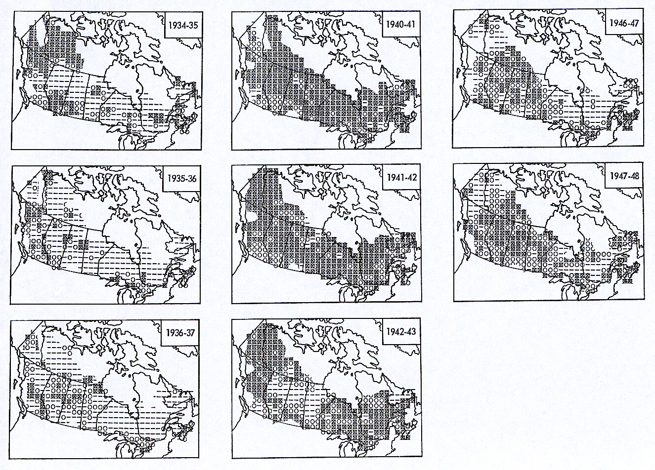
Figure 1. General trends in Snowshoe Hare population levels, 1931-32 through 1947-48. See text for explanation and key. [[For more detailed images of the figures above, click here and here.]]

[[p.156]] This map was constructed from 238 individual series lag values.

    Figure 3 is an isoplethic map of a surrogate used to help interpret relative amplitudes of the cycle in different areas. To derive this map, the proportions of the "no change" category noted at each grid cell location each year have been totalled for the seventeen year period. This value is an imperfect but useful surrogate for amplitude because it can be assumed that observers were likely to note "no change" more often for areas whose populations fluctuated less obviously. All 290 values were used to generate this map.

    Figure 4 is an isoplethic map of a surrogate statistic representing degree of non-random trend in the residuals of the detrended series. In most of the map, this can be considered to correspond to mean degree of cycle strength; in a few areas, however (notably the St. Lawrence Valley), trend was high despite lack of significant 8.9 years periodicity. This situation arises because the surrogate used here is the Durbin-Watson statistic, which measures trend only (and not cyclicity per se). Apparently, some parts of the study area were either undergoing long term population irruptions (unlikely) or were simply cycling in periods greatly varying from the 8.9 year national mean. Areas of the map that tested "no trend" at the 0.025 level of significance are labelled such; of the remaining areas, lower values signify clearer trend. All 290 values were used to generate this map.

    Despite the many possible sources of error in deriving these summary maps, it is felt they do a reasonably good job of representing the original data. A further validity check on the data of Figure 2 was carried out by averaging the values mapped on a province-by-province basis. The results are listed in Table 1. These results correlate very highly (r = 0.930) with Bulmer's

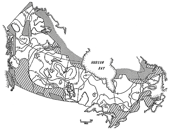
Figure 2. Geographic variation in Snowshoe Hare cycle phase, 1931-32 through 1947-48. Stippled shading signifies areas for which data were unavailable; diagonal shading signifies areas that did not cycle at the system mean of about 8.9 years period. See text for further explanation.

[[p. 157]]

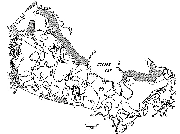
Figure 3. Geographic variation in Snowshoe Hare cycle amplitude, 1931-32 through 1947-48. Stippled shading signifies areas for which data were unavailable. Higher values here represent lower amplitudes; see text for further explanation.

(1974) provincial phase lag values for the Canada Lynx over the period 1919 to 1957, a good substantiation considering the two different types of data involved and the probability that Bulmer's results are spatially biased by his use of a national norm weighted unevenly by the varying sales volumes of furs for each province. In addition, data of Figure 3 show a trend similar to that subjectively assessed by Adams (1959). Still, it should be emphasized that only limited confidence can be attached to the specifics of pattern produced from such a short sampling period, regardless of the great cycle strength occurring in this case.

Discussion and Summary

    Subjective descriptions of the trends visible in Figure 1 accompany the original reports. A full analysis of these and the other data presented here will only be possible within the context of particular spatial-temporal modelling attempts; for the present, however, several general trends can be pointed out. The low amplitude / degree of cycling in south central Canada has been recognized for some time; this is also true for southern British Columbia and parts of the Maritime Provinces. Here, however, Nova Scotia tests as strongly cyclic, and with a large negative phase lag (These patterns were also discovered in the Lynx data analysis in Smith and Davis 1981). A second trend, recognizable in all three summary maps, is a tendency for patterns visible at the southern limits of range to be repeated at the northern limits; thus, phase lag tends to increase, amplitude to decrease, and strength of cycle to diminish geographically southward or northward away from a strip extending across central Canada (this impression has been confirmed in a trend surface analysis not presented here).

    A second set of interesting characteristics involves the rate of spread of the "wave" of population level change away from the main node in central Canada.

[[p. 158]]

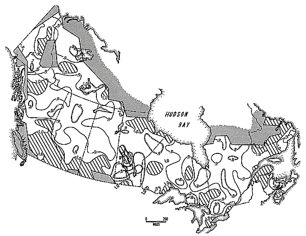
Figure 4. Geographic variation in non-randomness of Snowshoe Hare population trends, 1931-32 through 1947-48. Stippled shading signifies areas for which data were unavailable; diagonal shading signifies areas that did not pass the non-randomness test at 0.025 level of significance (and are mapped as values of 1.0 or greater). See text for further explanation.

_________________________

Table 1. Geographic variation in Snowshoe Hare cycle phase, 1931-32 through 1947-48, relative to the national mean, and aggregated at the provincial level. See text for further explanation.

Province                                Lag (in years)

Nova Scotia . . . . . . . . . . . . . . . .  -2.3
Manitoba . . . . . . . . . . . . . . . . . .  -0.8
Saskatchewan . . . . . . . . . . . . . . . -0.7
Alberta . . . . . . . . . . . . . . . . . . . .  -0.5
British Columbia . . . . . . . . . . . . . -0.1
Northwest Territories . . . . . . . . . 0.0
Ontario . . . . . . . . . . . . . . . . . . . . +0.4
Quebec . . . . . . . . . . . . . . . . . . . . +0.5
Yukon Territory . . . . . . . . . . . . . +1.5

First, it is apparent the manner of spread is not one of a simple node away from which diffuses a single wave of population change. Instead, minor nodes of change seem to appear in advance of the wave emanating from the main node, generating their own waves of advance. These eventually meet along "divides." This aspect of system organization seems worth further consideration, perhaps from an epidemiological perspective.

    Second, it appears the diffusion of population level change is in some way slowed by physiographic and / or ecological barriers. Figure 2 clearly shows the effect of the Rocky Mountains and the Great Plains on a wave of change emanating from its Boreal Forest origin. The meaning of this relationship is certainly [[p. 159]] not obvious. One might argue that it is indicative of a change in community interaction rates associated with lower population densities in suboptimal habitats, but the question then becomes how this spatial-temporal translation is effected and why it doesn't lead to an upset of standing phase relationships across the rest of the range. Moreover, it is difficult to defend central Alberta, for example, as being "suboptimal" habitat for the Snowshoe Hare. Nonetheless, this relationship does cast doubt on the likelihood of the simple external driving mechanism hypothesis of cycle causation, since it is difficult to consider this correlation between change in rate of diffusion and habitat change as a spurious relationship.

    In brief summary, this treatment has two general purposes. The first is to suggest the need for a view of ten-year cycle dynamics in which system-wide patterns are given primacy in the consideration of causal relationships. Failure to follow this route may result in much wasted effort as the effects of cycle operation are confused with its causes. The second is to produce from the best sources available a data base that can be used to support such spatial modelling attempts in whatever form they might take.

Acknowledgments

    I would like to extend my thanks to Dr. Arthur Getis of the Department of Geography, University of Illinois at Champaign-Urbana, for offering helpful suggestions during the course of this work, and to Mr. Phillip Schneider, for assistance in the preparation of the maps.

Literature Cited

Adams, L. 1959. An analysis of a population of snowshoe hares in northwestern Montana. Ecological Monographs 29(2): 141-170.

Bulmer, M. G. 1974. A statistical analysis of the 10-year cycle in Canada. Journal of Animal Ecology 43(3): 701-718.

Bulmer, M. G. 1975. Phase relations in the ten-year cycle. Journal of Animal Ecology 44(2): 609-621.

Butler, L. 1951. Population cycles and color phase genetics of the colored fox in Quebec. Canadian Journal of Zoology 29(1): 24-41.

Butler, L. 1953. The nature of cycles in populations of Canadian mammals. Canadian Journal of Zoology 31(3): 242-262.

Chitty, D., and H. Chitty. 1941. The Canadian arctic wild life enquiry, 1939-40. Journal of Animal Ecology 10(2): 184-203.

Chitty, D., and H. Chitty. 1942. The snowshoe rabbit enquiry, 1939-40. Canadian Field-Naturalist 56(2): 17-21.

Chitty, D., and C. Elton. 1937. The snowshoe rabbit enquiry, 1935-36. Canadian Field-Naturalist 51(5): 63-73.

Chitty, D., and C. Elton. 1938. The snowshoe rabbit enquiry, 1936-37. Canadian Field-Naturalist 52(5): 63-72.

Chitty, D., and C. Elton. 1939. The snowshoe rabbit enquiry, 1937-38. Canadian Field-Naturalist 53(5): 63-70.

Chitty, D., and C. Elton. 1940. the snowshoe rabbit enquiry, 1938-39. Canadian Field-Naturalist 54(8): 117-124.

Chitty. D., and M. Nicholson. 1941. The snowshoe rabbit enquiry, 1940-41. Canadian Field-Naturalist 57(4,5): 64-68.

Chitty, H. 1943. The snowshoe rabbit enquiry, 1941-42. Canadian Field-Naturalist 57(7,8): 136-141.

Chitty, H. 1946. The snowshoe rabbit enquiry, 1942-43. Canadian Field-Naturalist 60(3): 67-70.

Chitty, H. 1948. The snowshoe rabbit enquiry, 1943-46. Journal of Animal Ecology 17(1): 39-44.

Chitty, H. 1950. The snowshoe rabbit enquiry, 1946-48. Journal at Animal Ecology 19(1): 15-20.

Cole, L. C. 1951. Population cycles and random oscillations. Journal of Wildlife Management 15(3): 233-252.

Cole, L. C. 1954. Some features of random population cycles. Journal of Wildlife Management 18(1): 2-24.

Cross, E. C. 1940. Periodic fluctuations in numbers of the red fox in Ontario. Journal of Mammalogy 21(3): 294-306.

Elton, C. 1933. The Canadian snowshoe rabbit enquiry, 1931-32. Canadian Field-Naturalist 47(4): 63-69; 47(5): 84-86.

Elton, C. 1934. The Canadian snowshoe rabbit enquiry, 1932-33. Canadian Field-Naturalist 48(5): 73-78.

Elton, C., and M. Nicholson. 1942a. Fluctuations in numbers of the muskrat (Ondatra zibethica) in Canada. Journal of Animal Ecology 11(1): 96-126.

Elton, C., and M. Nicholson. 1942b. The ten-year cycle in numbers of the lynx in Canada. Journal of Animal Ecology 11(2): 215-244.

Elton, C., and G. Swynnerton. 1935. The Canadian snowshoe rabbit enquiry, 1933-34. Canadian Field-Naturalist 49(5): 79-85.

Elton, C., and G. Swynnerton. 1936. The Canadian snowshoe rabbit enquiry, 1934-35. Canadian Field-Naturalist 50(5): 71-81.

Finerty, J. P. 1980. The population ecology of cycles in small mammals: mathematical theory and biological fact. Yale University Press, New Haven.

Fox, J. F. 1978. Forest fires and the snowshoe hare-Canada lynx cycle. Oecologia 31: 349-374.

Getis, A., and B. Boots. 1978. Models of spatial processes. Cambridge University Press, Cambridge.

Huntington, E. 1945. Mainsprings of civilization. Wiley, New York.

Keith, L. B. 1961. Wildlife's ten-year cycle. The University of Wisconsin Press, Madison, Wisconsin.

MacLulich, D. A. 1937. Fluctuations in the numbers of the varying hare (Lepus americanus). University of Toronto Studies, Biological Series No. 43.

Moran, P. A. P. 1952. The statistical analysis of game-bird records. Journal of Animal Ecology 21(1): 154-158.

Moran, P. A. P. 1953. The statistical analysis of the Canadian lynx cycle. Australian Journal of Zoology 1(2): 163-173; 1(3): 291-298.

Moran, P. A. P. 1954. The logic of the mathematical theory of animal populations. Journal of Wildlife Management 18(1): 60-66.

[[p. 160]] Palmgren, P. 1949. Some remarks on the short-term fluctuations in the numbers of northern birds and mammals. Oikos 1(1): 114-121.

Rowan, W. 1950. Canada's premier problem of annual conservation: a question of cycles. New Biology 9: 38-57.

Smith, C. H., and J. M. Davis. 1981. A spatial analysis of wildlife's ten-year cycle. Journal of Biogeography 8(1): 27-35.

Received 10 September 1981
Accepted 30 August 1982