[[p. (i)]]

THE DYNAMICS OF ANIMAL DISTRIBUTION:
AN EVOLUTIONARY/ECOLOGICAL MODEL

BY

CHARLES HYDE SMITH

B.A., Wesleyan University, 1973
M.A., Indiana University, 1980

THESIS

Submitted in partial fulfillment of the requirements
for the degree of Doctor of Philosophy in Geography
in the Graduate College of the
University of Illinois at Urbana-Champaign, 1984

Urbana, Illinois

[[p. (ii)]]

THE DYNAMICS OF ANIMAL DISTRIBUTION: AN EVOLUTIONARY/ECOLOGICAL MODEL

Charles H. Smith, Ph.D.
Department of Geography
University of Illinois at Urbana-Champaign, 1984

    Investigators have sometimes assumed that the factors underlying animal distribution are too complex to lend themselves to normative modelling. In this work, a model of environment and community interaction is constructed which lends itself to the latter kind of interpretation. It is posed that spatially-varying rates and magnitudes of availability of moisture at given locations act as stresses on the nature of community infrastructure, and secondarily on the rates at which new populations may become integrated into these. Populations are thereby viewed as tending to change range in common directions, though at overall rates remaining peculiar to each. This interpretation is shown to lend itself to a synthesis of ecological and evolutionary approaches to distributional controls, and to suggest some novel viewpoints on the nature of evolutionary change and ecological interaction in general. The model is tested through a series of empirical studies of distribution patterns of all mammal and herptile species inhabiting the middle one-half of the United States. The results of the tests are in general consistent with expectations; for example, highly stressed community structures are shown to be correlated with smaller range sizes, greater variation in range sizes, and direction of dispersal. Spatial variation in stress magnitude is also shown to influence rates of faunal interaction between locations. The study concludes with a discussion of means whereby ecological modes of analysis can be extended to the study of evolutionary change over longer periods of time through the present model.

[[p. iii]]

ACKNOWLEDGMENTS

    The author is indebted to a number of individuals who contributed time and attention to the development of this study. I should like to individually thank Gila Shoshony, Richard Chorley, Dave Swofford, Leigh Van Valen, Wayne Wendland, Donn Rosen, Torsten Hägerstrand, James Burt, Bruce Hannon, Judith Hill, Gareth Nelson, John Endler, and Mindy Wade for their various kinds of input, and to congratulate the members of my Committee for having the patience and confidence to see this work through to its completion.

[[p. iv]]

TABLE OF CONTENTS

Section                                                                                                                                     Page

I. INTRODUCTION . . . . . . . . . . . . . . . . . . . . . . . . . . . . . . . . . . . . . . . . . . . . . . . . . . . . 1

II. CRITICISM OF THE LACK OF EMPHASIS ON SPATIAL INTERACTION
MODELLING IN ZOOGEOGRAPHY. . . . . . . . . . . . . . . . . . . . . . . . . . . . . . . . . . . . . .  9

        An Historical Perspective on Trends of Study in Zoogeography . . . . . 9

Two Recent Innovations in the Study of Zoogeographic Patterns . . . . . 20

A Summary of Past Perspectives . . . . . 28

The Present Study . . . . . 31

III. MODEL DERIVATION: SYSTEM FRAMEWORK. . . . . . . . . . . . . . . . . . . . . . . . . .34

Energy and Mass Flow Through the Earth's Surface System . . . . . 34

System Controls and Exchanges . . . . . 37

Spatial Interaction and Evolution . . . . . 46

Spatial Interaction in the Community Context . . . . . 55

IV. SPATIAL INTERACTION AND RANGE CHANGE: AN INNOVATION
DIFFUSION MODEL. . . . . . . . . . . . . . . . . . . . . .. . . . . . . . . . . . . . . . . . . . . . . . . . . . . .67

Innovation Diffusion Models . . . . . 67

Range Change Modelled as Innovation Diffusion . . . . . 73

V. FITTING THE MODEL FOR EMPIRICAL PURPOSES . . . . . . . . . . . . . . . . . . . . . . 80

A Measurable Surrogate for Stress . . . . . 80

Data Used in the Empirical Studies . . . . . 90

VI. SOME EMPIRICAL TESTS OF THE MODEL . . . . . . . . . . . . . . . . . . . . . . . . . . . . . 98

Introduction . . . . . 98

Analysis One . . . . . 104

Analysis Two . . . . . 107

Analysis Three . . . . . 110

Analysis Four . . . . . 112

Analysis Five . . . . . 114

Analysis Six . . . . . 115

Analysis Seven . . . . . 118

Analysis Eight . . . . . 122

Analysis Nine . . . . . 124

Analysis Ten . . . . . 126

Analysis Eleven . . . . . 129

Summary . . . . . 130

[[p. v]]

VII. EVOLUTION AND THE RECURSIVE DEVELOPMENT OF DISTRIBUTION
OF DISTRIBUTION PATTERNS . . . . . . . . . . . . . . . . . . . . . . . . . . . . . . . . . . . . .136

Vicariance Events, Speciation, and Evolutionary Equilibrium . . . . . 137

Adaptability and the "Adaptive Landscape" . . . . . 158

The Analysis of Cumulative Pattern Development . . . . . 163

Altitudinal Zonation and Relict Populations . . . . . 173

A Regional Case Study . . . . . 179

Simulation Studies . . . . . 186

APPENDICES . . . . . . . . . . . . . . . . . . . . . . . . . . . . . . . . . . . . . . . . . . . . . . . . . . . 191

REFERENCES . . . . . . . . . . . . . . . . . . . . . . . . . . . . . . . . . . . . . . . . . . . . . . . . . . 220

VITA. . . . . . . . . . . . . . . . . . . . . . . . . . . . . . . . . . . . . . . .. . . . . . . . . . . . . . . . . . . 241

[[p. 1]] I. INTRODUCTION

    Biogeography is often considered one of the most highly interdisciplinary sciences. Its complexities have sometimes prompted its students (see Myers, 1937: 340; Darlington, 1957: ix; Wilson, 1970: 1193; Elton, 1958: 34-35; Davies, 1961: 416) to complain that no one person can master all the cognate studies necessary to a full understanding of its subject matter, the distribution of organisms. Many have nonetheless entered into speculation regarding the causes of existing distribution patterns. Related discussions have usually arisen as a logical outgrowth of interest in the evolution and systematics of particular organismal lineages (the "geographical zoology" of Wallace: 1860, 1876) or through a desire to view community conditions at a given location in somewhat more general historical (Wallace's "zoological geography": 1860, 1876) and/or environmental (MacArthur's "geographical ecology": 1972) terms.

    Regardless of the particular motivation for carrying them out, biogeographic studies have usually had as their goal increasing our knowledge of the biology of organisms (or groups of organisms). It is therefore not surprising that there is little theory that can be identified as elementally "bio-geographic;" that is, whose level of departure is organism-environment interrelation as opposed to organisms alone. This "geography as handmaiden to science" use of distributional data is not without its drawbacks. When the links among distribution, environment, and organismal function and change are stated in non-recursive terms, the resulting geographic perspective is predictable: distribution characteristics are demoted to the status of results--that is, to a kind of knowledge that cannot be used to examine future system change. Moreover, an [[p. 2]] idiographic position is forced. If one begins with the proposition that each population of organisms occupies unique and discrete spatial and temporal coordinates in the history of life, it is difficult to view associated causal conditions as being other than population-specific.

     While it is often useful to think in population-specific terms, it seems counterproductive to argue that the study of organismal distribution must proceed from this starting point alone. At best this attitude is narrow-minded; at worst it is inconsistent, because it leads to the picture of a biosphere ordered at the level of its parts, but not in sum. We do not consider the concept of natural selection internally contradicting merely because the exact forces of selection on each population are different; neither should we dismiss the idea that the spatial distribution of populations might be interpreted as a single kind of response to some set of environmental influences. The natural selection model has provided a means whereby biological diversity can be ordered in logical fashion; similarly, we might be able to develop a general spatial interaction model relevant to the depiction of organismal distribution and its characteristics of change through time. Two main reasons can be identified for believing that the distribution of organisms (and the evolution of distribution) might be dealt with on such a wholly normative basis.

    First, if we acknowledge that there has been a general ordered change in the level of complexity of organisms, we should also suspect that this has borne an ordered relationship to the general spatial setting within which it has taken place. The reason for this is fundamentally that the earth's surface is limited in extent, a constraint leading to a continual replacement of older forms by newer ones as lifestyle opportunities come and go. This process goes on and on, independent of the particular [[p. 3]] organisms involved. It is unthinkable that the spatial conditions which sponsor such turnover of populations can be considered as less than the necessary and sufficient causes for the characteristic patterns of distribution that are produced. It seems difficult to argue that a world with spatially-unlimited resources would promote competition for these; needs that could not be met at one location could always be satisfied simply by going elsewhere. A spatially-limited environment, on the other hand, stimulates competition by rewarding with survival those organisms that can most efficiently utilize available resources (Darwin, 1859a, 1859b; Wallace, 1859; Tilman, 1982).

    The fact of a generalizable competition process among organisms provides a normative basis for the theory of natural selection. But while the results (biotic diversity) of competition/natural selection--or whatever biological evolution-inducing process we wish to imagine--can easily be understood to exist "in space," it is quite another matter to try to use such aspatial understandings to predict specifically what the spatial relationships constituting "in space" should be. There is nothing explicit in biological evolution models that leads, for example, to an understanding of the way instances of competition at a given time and place feed back to affect the nature of competition at later times in other places. To say simply that there is a "geographic component" to the process of evolution is to say nothing; where the matter of interest is the diffusion of an influence through space and time, this component and its recursive underpinnings must be specified to make possible hypothesis-testing and predictive science. Preferably, we should think in causal terms in this endeavor. Organisms are non-randomly distributed, and we should therefore expect the influences contributing to this order to be themselves [[p. 4]] non-randomly distributed in space (Getis and Boots, 1978; Baker, 1982; Sheppard, 1979; Rich, 1980); that is, to be linked to "preferred" routes through time and space for organismal change. Evolution is not just a process that takes place "in space", it is a process that takes place because of (or even as) space. Any regularities in the evolution of organisms should be referable to the spatial relationships promoting them.

    Second, evolutionary outcomes are as much a function of input from the inorganic world as they are input from the organic world. Lest limited material resources be rapidly depleted and evolution abruptly stop at an early stage (see Hanson (1977), Cloud (1974, 1976), and Windley (1975) for related discussions), the first requirement of an evolutionary process occurring within a finite space is that it involve mechanisms by which resources can be used over and over, each time in a slightly different way, and often (or usually) by many different types of organisms. Nothing that is alive remains so for very long; indeed, even the elements comprising individual organisms when they are alive are continually being replaced. Given the fact that living things share materials that are both necessarily derived from the physical environment and passed back to it for recycling ("turned over"), regularities in the spatial structure of the physical environment must at some level be reflected in the way organisms evolve. Spatial variation in the way elemental resources turn over, for example, is certainly linked to spatial variation in competition regime types (E.P. Odum, 1969, 1971; Tilman, 1982; Hutchinson, 1964, 1978; Ford, 1982). Inasmuch as evolution: 1) is an irreversible process (Conrad, 1983; Prigogine, 1961) and 2) is characterized by changing patterns of interaction occasioned by the mobility of organisms/populations, such constraints on biological evolution in one setting can be expected to have delayed impact [[p. 5]] on other settings at later times. The study of the properties of organic diversity should therefore also be concerned with the regular way in which the unfolding of that diversity is constrained and/or enhanced by the distribution properties of exogenous physical influences. To exclude a consideration of the latter from biogeographic modelling is to make the mistake of thinking that the biosphere is an isolated system.

    The present work is organized in three parts. The object of the first (Chapters II through V) is to develop a model of biotic-abiotic interaction that can serve as a generalized starting point for the study of the distribution of animal (or plant) populations. The first step toward this goal is a brief treatment (in Chapter Two) of biogeography's major philosophical positions of the last two hundred years; the reason for this analysis is not so much to criticize these with respect to their present domains of application, but instead to point out their inflexibility regarding the study of distribution as spatial interaction (see below for a definition of this term). From this beginning a model is developed which, it is hoped, will prove more adaptable in this regard.

    A major portion of the first part of the work is devoted to characterizing changing distribution patterns as the reflection of a general progression in the ecosphere toward steady-state conditions. Two key elements in the discussion are the development of the concept of the "stress field," and an emphasis on community evolution-level constraints on range change in individual species populations. The stress field concept is introduced in an effort to specify how spatial variation in a critical physical environmental factor might influence range change in populations of organisms. It is argued that spatial variation in this factor must affect rates of "flow" (range change) of species populations--and therefore their [[p. 6]] collective spatial pattern--accordingly; a simplistic but somewhat useful analogy may be drawn with the relationship between shallow ocean bottoms of varying depth and the surface wave front patterns relatable thereto. The community level emphasis is productive in that community change is more easily linked to combinations of historical and environmental variables than is the evolution of an individual population to these; whereas the historical interaction of environment and populations is only implicit in the biology of speciation and but remotely connected to phylogenetic studies, the historical interaction of environment and communities might be explicitly interpreted as rates of integration and loss of populations into/from the latter. The "flows" of populations implied can then be dealt with on normative terms; likewise, the distribution patterns resulting. The spatial interaction process argued to underlie this flow is represented here through a modified innovation diffusion model in which the rate of "acceptance" of new populations into a given community structure is viewed as being in effect constrained by the local characteristics of the stress field.

    An inherent feature of the discussion is that most of its conclusions arise from deductive arguments pertaining to systems concepts only indirectly related to the mainstream of biological research. Where possible I have attempted to provide a biological context, but at no point should the reader forget that the object of the work is to deduce from general system principles--and not the characteristics of specific organisms, populations, or communities--conclusions leading to predictions regarding the nature of distribution patterns. I am, in fact, logically obliged in all but a few instances to refrain from introducing any information gained from the study of the biology of organisms into my arguments; the specific reason for this [[p. 7]] will only become apparent by the third chapter. The general rationale is to provide a discussion in which process terms and structure terms are kept separate from one another as much as possible. I believe, in concert with other opinion (see, for example, Grene, 1971; Eldredge, 1981; Gould and Lewontin, 1979; Washburn et al., 1963; Ball, 1983; Ghiselin, 1966, 1984; Teichert, 1958; Hull, 1974; Gould and Vrba, 1982), that such separation is central to reducing the regressive thinking that can result when terms describing causal structures are synonymized with those referring to morphological structures. In Chapter III this strategy--a deliberate avoidance of individualistic "functional statements" (Nagel, 1961; Ruse, 1973)--will be shown to have implications that are both philosophically attractive and scientifically useful.

    Much use of the term "spatial interaction" is made in this work, especially in the model development of the first part. We can define spatial interaction as both a general process and the events contributing to that process. In general terms, it can be viewed as a system of flows of various magnitudes connecting locations in space. The individual events that maintain such flows can be understood to have two fundamental properties. First, they must be recurring; i. e., their instances of occurrence in time and/or space must be non-unique and non-random. Second, they must occur in response to causal associations that develop between or among comparably-defined entities. Recurrence of events is a property needed to specify persistence; without the latter it is impossible to recognize the notion of "flow" or a system maintained thereby. The "comparably-defined entities" clause represents an effort to restrict the depiction of events to unambiguous cause and effect relationships (Nagel, 1961; Wolvekamp, 1982). I would argue, for example, that wars are fought [[p. 8]] between nations or the people making up nations, but not between one nation and the people making up another. Similarly, it is logically difficult to specify terms of causality between cells and organs or between organisms and whole communities because the entities involved are defined in such a way that they occupy the same space at the same time. A good example of spatial interaction in both its macro- and micro-level forms is afforded by international trade of goods. Here, the flows are stated in terms of "commerce" (dollars exchanged) among countries, and the events making these up, in terms of individual instances of purchase of goods.

    The second part of the work (Chapter VI) relates the results of some empirical tests of the ideas developed earlier. The fundamental tenets of the model are combined in such a way as to yield predictions regarding the characteristics of pattern of distributional ranges (and boundaries thereof) in a particular study area. These predictions are then tested through the aid of univariate and multivariate statistical methods.

    In the last part (Chapter VII), some topical issues within biogeography are addressed from perspectives grounded in the current model. Much of the early discussion in this section is of speculative nature, but in addition tests of some of the ideas presented are suggested and further empirical studies bearing on relevant matters introduced. The general object of this third part is to show that the model developed here can be used to consider longer-term implications of the evolutionary/ecological process underlying distribution patterns as well as its more immediate dynamics.

[[p. 9]] II. CRITICISM OF THE LACK OF EMPHASIS
ON SPATIAL INTERACTION MODELLING IN ZOOGEOGRAPHY

An Historical Perspective on Trends of Study in Zoogeography

    Two of the most fundamental questions asked by zoogeographers are how populations of animals have come to be located where they are, and why those populations do not exist in other places (where one might for various reasons expect to find them). The complementarity of these two questions seems obvious enough now, but before the 1700's, not enough was known about the distribution of animals to even suggest they should be asked. In that century, two important developments took place.

    First, it was discovered (thanks to the collective efforts of field naturalists) that ecologically-similar but geographically-distant areas tended to be populated by entirely different suites of species. This fact, first described in detail by Buffon (Buffon, 1749-1803; see discussion by Nelson, 1978; Nelson and Platnick, 1981) and now known as "Buffon's Law", was instrumental in forcing naturalists to think more carefully about the causal factors underlying the present distribution of organisms. Around the same time, knowledge of the fossil record began to congeal into a systematic understanding of the history of life. Paleontology suggested three further bits of information to be taken into account before the present distribution of animals could be understood: 1) that at present many organisms cannot be found in places where they obviously once flourished, 2) that most forms now living do not show up as fossils, and 3) that most forms known through fossils seem not to be represented by living organisms.

    With the latter clues in hand, naturalists began to consider whether [[p. 10]] the biosphere might change through time in a fashion explaining Buffon's Law. There appeared to be two ways that such change could take place. The more conservative explanation--because it didn't conflict with Biblical teachings--was that distributional ranges alone vary with time. As the world was more fully explored, however, it became apparent that many forms known only as fossils were now truly extinct. Moreover, presently-existing forms seemed to appear on the average rather late in the fossil record. This latter fact suggested a second possible vehicle of change for the biosphere: that organisms themselves might have come into being at various points in time. Attention was drawn to how this might take place.

    Two general kinds of causal models seemed appropriate. In the first, environment was viewed as forcing change; that is, as somehow directly specifying those adaptations that were needed to survive. The same kind of determinism could be invoked to explain distributional range changes in the shorter term sense; were the climate of an area to rapidly change, many existing occupants would be rendered unfit and forced out. On the other hand, it was also possible to imagine range shifts as being adaptive rather than forced; that is, as constituting a means of exploiting new opportunities. The trouble with this approach was that no one could propose a mechanism to explain constructive responses that was not inherently teleological (as had been, for example, the earlier "Great Chain of Being" understanding: Lovejoy, 1936). As a result, the first organismal change models proposed followed the idea that environment--and climate in particular--must "shape" organisms in a manner allowing them to exist under given conditions. This view was sponsored by most of the important thinkers of the period, notably Buffon (1749-1803), Maupertuis (1750), Forster (1777), Malthus (1798), Fabricius (1804), Montesquieu (1802), the older [[p. 11]] Candolle (1817, 1820), and, most of all, Lamarck (1809), who proposed a specific mechanism for organic change: the adoption of acquired characters.

    Not everyone during the pre-Darwinian period was satisfied that organic change provided a satisfactory base for explaining current distribution characteristics, however. Many ignored both Lamarck and fossil evidence (Brooks, 1984; Kinch, 1980) and continued to believe that present patterns of diversity were simply a function of Divine Will, a position seemingly supported by the existence of disjunct distributions (Kinch, 1980). Some (e.g., P.L. Sclater, 1858), seeking a descriptive understanding of the Creation, adopted a quasi-scientific approach to the matter by systematically searching for "Centers of Creation" through faunal region delineation methods. Others (e.g., Charles Lyell, 1830-1833, 1972) were willing to accept the Creationist stance but still believed that the matter could be addressed using a scientific approach extending beyond mere description. To complicate matters further, some (e.g., Edward Forbes, 1846) defended the notion of Centers of Creation while at the same time arguing that post-Creation dispersals had rearranged original patterns of distribution.

    The introduction of the Darwin/Wallace theory of natural selection (Darwin, 1859a, 1859b; Wallace, 1859) accelerated discussion further. Natural selection avoided an explicitly teleological stance on organic change but was still flexible enough to treat adaptation as a dynamic response to environmental/community conditions. Wallace (1860, 1863, 1866, 1869, 1876, 1880) led in applying the natural selection concept to the realm of zoogeography per se; by methodically drawing together the existing data of several different fields (notably, climatology, paleontology, paleogeography, and oceanography) and considering this information in light [[p. 12]] of past and present distributional records, he was able to evaluate the relationship of spatial differentiation to evolution (George, 1964; Smith, 1980, 1984; Fichman, 1977, 1981; Brooks, 1984). Specifically, once it was granted that organisms could evolve and had (varying) powers of dispersal, their occurrence in different regions over spans of time could be viewed as initial evolutionary events followed by dispersals away from place of origin (oftentimes leading to subsequent radiations in the new areas reached). This approach could be used to understand the evolution of biogeographic regions (and, ultimately, Buffon's Law), since periods of geographic isolation (whether locationally- or environmentally-induced) would prevent an area from receiving flows of new outside forms, thereby promoting the development of unique faunas.

    The Darwin-Wallace synthesis was not immediately embraced by all workers interested in the study of distribution. A number continued to favor the earlier position that climatic influences largely dictate how (and where) a particular organism could evolve. This was seen as being especially so in areas of harsh environmental conditions (such as the arid American Southwest). The underlying logic was reasonable: it was difficult to believe that an organism unadapted to a certain climate would be able to disperse through it or into it. This argument had also been used by Agassiz (1850) and others to defend Creationist views on animal distribution (and is still used from time to time in modern contexts: note Lovtrup's (1981) criticism of Eldredge and Gould, 1972). This understanding was not as evolutionarily short-sighted as it may initially appear, since most of its advocates also believed in the inheritance of acquired characters (the "neo-Lamarckism" especially championed by Lester Ward, Edward Cope and Alpheus Hyatt--see Campbell and Livingstone, 1983; Livingstone, 1984). [[p. 13]] Climate could thus directly induce evolution (at the same time, however, the role of dispersal was rendered somewhat obscure).

    These leanings extended to the way some thought zoogeographic regions should be portrayed. Allen's (1871, 1877) scheme, for example, was more of an ecological classification than a zoogeographic one, and was heavily criticized by Wallace (1876) and others for ignoring the evolutionary interrelationships of faunas. Merriam's "life zones" model (1890, 1894, 1898) was a similar effort to treat regionalization from a limiting factors perspective. Around the same time, the Russians (starting with Dokuchayev, 1951) began developing the analogous system of "zonal" classification, use of which has continued to the present day (Stegmann, 1938; Grigor'yev, 1936; Grigor'yev, 1961; Matveyev, 1972; Grishankov, 1973; Berg, 1947-1952).

    The ecological approach to zoogeographic classification competed well with the historical approach-based Sclater/Wallace system (Sclater, 1858; Wallace, 1876) among biogeographers of the late nineteenth century. But even before the end of the 1800's it had become apparent that neither alone provided a wholly adequate basis for the study of distribution (Gill, 1885; Blanford, 1890). Lydekker (1896), apparently rediscovering the work of Candolle (1817, 1820), made an important attempt at reconciliation with his differentiation between the notions of "distributional area" and "station." This separation of concepts provided a useful tool through which the properties of distribution could be viewed from either a historical or ecological, respectively, perspective. Shortly thereafter, the acquired characters approach began to fall into general disfavor, and the environmental determinists were faced with attributing greater importance to the role of natural selection in evolution and dispersal or coming up with a better causal model than natural selection. Matthew (1915) eased many out [[p. 14]] of this dilemma by forging an argument for the role of dispersal in evolution that linked the nature of present and historical organismal distribution data to the distribution of climatic conditions. Most, unfortunately, found Matthew's correlations-based discussion so seductive that in the long run the development of biogeographic thought may actually have been retarded by its early uncritical acceptance (see comments by Croizat, 1981; Nelson, 1978).

    Around the same time, the pace of investigation of distributional anomalies began to increase, partially in response to the comments of Wallace (Wallace, 1863, 1876, 1894; see Fichman, 1977, 1981). The elucidation of past and present constraints on avenues of dispersal became a major focus of interest. Such efforts often reduced to explaining present patterns via simplistic paleogeographic reconstructions. Many of these attempts were permeated by poor logic. For one thing, supporting geologic evidence was often meagre or entirely lacking--as in the land bridge theories of Joleaud (1924) and Ortmann (1910). Perhaps more embarrassing were the logical inconsistencies created by these ad hoc explanations. For instance, land bridge dispersal routes sometimes postulated to explain a supposed extension of range of certain organisms from place A to place B were often unable to reconcile the curious fact that no dispersals by other species had apparently taken place in the opposite direction. Simpson (1940, 1943) provides wonderful critiques of such excesses. Through the critical efforts of Simpson and others (for example, Schuchert, 1932; Myers, 1937; and Darlington, 1938) the transparency of many such ad hoc explanations was justly exposed.

    The nineteenth and twentieth centuries have also witnessed a long line of progress in the study of the microclimate interface between organism and [[p. 15]] environment. Following the initial work of Liebig (1840) and extensions by Shelford (1911, 1913), the theory of limiting factors was expanded in many directions to account for all kinds of ranges of organismal tolerance of the environment. At times, biogeographers have attempted to apply such knowledge directly to a causal understanding of regional distribution patterns, but nothing of much worth has ever resulted (typical was the failure of Merriam's "life zones" approach). Unfortunately, while telling us a great deal about what evolution has accomplished at the individual level, the limiting factors/physiological ecology perspective falls short of identifying the role in evolution of causal processes of spatial and temporal magnitude greater than those referable to the lives of individual organisms. Gates (1970: 132) has stated:

"I have contended for a long time that if I knew the properties of a particular animal I could predict the climate within which the animal must live in order to remain in thermodynamic equilibrium....This will give us insight to the geographical distribution of animals throughout the world and their adaptation to various climates."

But Gates, a foremost modeller of the organism-environment interface (for example, Gates, 1962, 1980) does not consider the matter of the relation of organic change to geographical distribution. In his work (and that of many others: for example, Geiger, 1955; Shelford, 1911; Taylor, 1970; McNab, 1971, 1979, 1982; Kleiber, 1932; Vernberg, 1975; Scholander et al., 1950; Lowry, 1970) the focus is on the individual organism; again, this systems-analytical approach ignores larger-scale spatial and temporal components of the biological continuum. As a result, environmental, community, and population turnover properties (not to mention the evolutionary interaction of these) are not dealt with.

    The extension of the limiting factors approach to the modern theory of [[p. 16]] the niche (MacArthur, 1955, 1968; Hutchinson, 1957, 1959; Savage, 1958; Preston, 1960, 1962; Whittaker, 1953, 1962) has been based largely on the idea that an organism's (or population's) sphere of activities can be expressed as a hypervolume defined by ranges of values of physical and biological variables. While this development opened the way for more sophisticated treatments of population- and community-level processes (examples include: 1) the gradient analysis studies of Whittaker and his followers: Whittaker, 1967, 1973, McIntosh, 1967; 2) ecological succession modelling: Horn, 1975, 1976, Odum, 1969, Pickett, 1976, Gutierrez and Fey, 1980; and 3) extensions of the general Lotka-Volterra model: May, 1976, Gilpin, 1975, Pielou, 1969, Schoener, 1976), it has been less successful in suggesting biogeographic models. This is probably because it is no less difficult to view an organism's niche as being other than the individualistic result of the evolutionary process that put it where it is than it is its suite of adaptations. Gould and Lewontin (1979) argue in this context that it is unproductive to dwell on the study of "unitary traits" because it becomes too easy to construct credible but untestable "just-so stories" accounting for these. As a result, evolution is trivialized, and possible cumulative structural controls on the general process of selection are ignored. This argument would seem to hold for the biogeographic context as well. When distributional range is viewed as being limited by combinations of factors specific to given populations, we are restricted to making geographical associations that can be stated only as ecological truisms or simple historical narratives (after Goudge, 1961). In so doing we also trivialize the meaning of geographical distribution: uniqueness is emphasized and we ignore the possibility that the individual distributional histories we can document may have evolved in response to the [[p. 17]] operation of non-population- and location-specific environmental influences.

    I therefore believe that a dynamic and generally applicable model of the way distribution patterns evolve cannot be based on information derived from the study of the particular biological properties of organisms (i.e., their niche and phylogenetic relationships, morphology, and behavior); such attempts invariably force us into thinking in terms of correlations with the environment rather than recursive processes (a similar argument has been posed by Maze and Bradfield, 1982). Yet zoogeographers continue to begin their comparative historical and ecological studies of distribution with the study of the biological attributes of organisms. This approach is reasonably effective when interest centers on historical reconstruction of distributional change or ecological understandings of the relation between adaptation and environment, but is not so useful to promoting a synthesis of these two approaches. As a result, the spatial interaction processes directly linking ecological constraints to historical outcome are invariably weakly specified in biogeographic studies (a complaint also raised by Deignan, 1963; Croizat, 1958). As a substitute, pseudo-terms such as "dispersal" have been invented that put labels on distributional change rather than explicate same; that is, that reduce to narrative description the structural dynamics of the spatial interaction underlying such change. (Nelson (1983: 484) makes a similar point regarding the use of descriptive terminology in evolutionary studies.)

    As long as narrative remains the preferred means by which the nature of distributional patterns and change in same is specified, I believe it cannot be stated fairly that the level of zoogeographic thought has significantly advanced beyond Wallace's synthetic philosophy of the mid-nineteenth century (see Gould and Lewontin (1979) and Nelson (1983) for further criticism [[p. 18]] linking Wallace to the present discussion).

    There seem to be two immediate and related factors contributing to this impasse. First, it is now virtually taken for granted by most historical zoogeographers that the evolution of distribution patterns is to be viewed in terms of the individual evolutionary histories of those organisms involved. Nelson (1983: 490), for example, referring to "future prospects" in biogeography, comments: "The methodological approach will employ cladistics....The empirical approach (will concern) the use of biogeographical data as viewed in the cladistic aspect." I have already suggested that approaches beginning with the study of organismal traits are more likely to conceal the interaction processes serving evolution than explicate these. But this position can also be criticized on at least two other grounds. For one, it is in no sense obvious that models of change at the organismal and population levels will appropriately serve a synthetic understanding of distribution patterns (for example, the way regional faunas and floras evolve). Uncritical application of theory in this direction invites the individualistic fallacy, and criticisms of the type offered by Gould and Lewontin (1979). Workers involved in suborganismal-level research seem to have perceived an analogous danger and have responded accordingly: for example, by largely abandoning the idea of natural selection in the development of their problem-solving approaches. Instead, they treat it as a unifying concept to which they can refer as a means of relating the processes they study to other contexts (Kimura, 1983a). We should expect no more from evolutionary theory--or any other aspatially-based understanding--as a contributor to zoogeographic understandings.

    A second criticism regards the overall strategy/object of historical biogeography. It has been suggested to me by members of the historical [[p. 19]] school that recent innovations (see below) in the methodology of zoogeography will make possible more accurate reconstructions of the history of past speciation events and associated distribution pattern evolution than had ever been thought possible (see also the comments of Platnick and Nelson, 1978). But what then? While this effort cannot in itself be condemned, it reflects something of a case of short-sightedness on the part of the historical school. Both geographers and historians are well acquainted with the long-term results of pursuing lines of study focusing on results rather than underlying generative processes: a general dwindling of interest. Geographers, at least, have been able to re-orient themselves toward process-oriented approaches (James, 1981; Johnston, 1981; 1983; Amedeo and Golledge, 1975; Davies, 1972; Griffith and Lea, 1983); historians, however, have had greater difficulty (Graubard, 1972; Gilbert, 1972; Cochran and Hofstadter, 1960). It is worthwhile to note, moreover, that geographers have found descriptive historical approaches unprofitable bases for normative modelling (note the present rejection, for example, of the geographical cycle notion of Davis (1899), the sequent occupance model (Mikesell, 1973), and the finalistic plant succession interpretations of Clements (1916)). An explanation for this is suggested in the following passage from Maruyama (1963: 174):

"....(when) the rules (of system evolution) are unknown, the amounts of information needed to discover the rules is much greater than the amount of information needed to describe the rules. This means that there is much waste, in terms of the amount of information, in tracing the process backwards than in tracing it forward."

In short, normative models provide more efficient description than does historical narrative. Thompson (1983: 168-169) has even gone so far as to argue that "generalizations which relate some present property to a [[p. 20]] developmental sequence of properties or events" (i.e., 'historical laws') "are not possible within current biological theory."

    Efficient description, however, does not necessarily provide the kind of detail that is needed for many purposes of investigation (especially where regional evolution is involved). Ideally, we might wish to develop zoogeographic theory that is efficient in its generalization of process yet still capable of specifying unique conditions of interaction. This brings up the second problem that has retarded expansion of zoogeographic theory: the lack of a synthesis of historical and ecological approaches that can be used at an elemental level in the study of animal distribution patterns (see relevant remarks by Endler, 1982b; Eldredge, 1981). On the basis of preceding comments, it seems that such a synthesis should be forged from: 1) efficient treatment of the general processes organizing distribution patterns; 2) an awareness of the need to specify not only that such processes "occur in space," but precisely where in space under any given conditions as well; and 3) a distributional (spatial) emphasis rather than an organismal (biological) emphasis. Regarding the third element, it must be added that this emphasis should be capable of producing lines of thought that can be related to properties of biological organization (in a commensal fashion similar to that which has been so successful in, for example, the allied fields of genetics and population genetics).

Two Recent Innovations in the Study of Zoogeographic Patterns

    The preceding comments, while critical in some instances, are not meant to suggest that zoogeography has been a static field of late. On the contrary, over the last fifteen years or so interest has risen to a relative level nearly comparable to that of the time of Darwin and Wallace. [[p. 21]] Nonetheless, I would argue that this interest can be attributed more to methodological advances and refinements in the available databases (for example, the effect that the development of plate tectonics theory has had on our reconstructions of paleogeography) than it can theoretical advances. It is important to understand the difference here; to improve the means through which data are reconciled is not necessarily--or even usually--equivalent to providing a new interpretative context for these. This is true whether or not such methods have genuine explanatory power, since explanation can be provided just as easily in immediate terms as in more general ones. (Kuhn (1962: Chapters Four and Five) develops a similar argument.) These remarks especially apply to the two most important recent contributions to the method of zoogeographic inquiry: the "island biogeography" of MacArthur and Wilson (1963, 1967) and "vicariance biogeography." A few comments on each should be made before we proceed.

    MacArthur and Wilson's equilibrium theory of island biogeography comes closer to making normative statements about observed patterns of distribution than has any other work within the discipline of biogeography. It describes--through logic combining gravity model (distance-decay) principles and the notion of the evolution over time of an equilibrium between colonization and extinction rates--the diversity characteristics of biota on islands of varying sizes located at varying distances away from an assumed source of biotic propagules. As such, it provides a means of explanation that, importantly, is specific to neither setting nor organism type (Endler, 1982a). It has been applied and extended in many important ways; here, however, we must be concerned more with its main relevant limitations.

    First, its sphere of application extends only to island or island-like [[p. 22]] situations (for examples of studies concerning the latter see Brown, 1971; Vuilleumier, 1970; Carlquist, 1974; Simberloff, 1974; Vuilleumier and Simberloff, 1980): generalization of the approach to continental conditions is not implicit (but see Smith, 1983b). Second, it implicitly treats islands as communities ipso facto; that is, the only condition of entry of colonizing groups into community infrastructure is the mere ability to physically reach and remain there. Distance and area factors become the main subjects of analysis, and while these can be used to provide portrayals of diversity relationships (May, 1975; Simberloff and Wilson, 1970; Simberloff, 1974; MacArthur and Wilson, 1967; Diamond, 1972; Preston, 1962; Connor and Simberloff, 1978), they are less useful to studying organism-environment interactions leading to evolution at the individual population level. Regarding this last point, Williamson (1981: 82-84) has outlined four basic weaknesses inherent in the theory in its original form: 1) it deals "explicitly only with the numbers of species, not with the numbers of individuals in species;" 2) the species of a given system of islands are dealt with as a lump sum, rather than as a functioning community; 3) historical factors influencing given sets of conditions are not taken into account; and 4) it does not take evolution in situ into account. Moreover, Williamson presents evidence that the main predictions made by the theory have not always been borne out in empirical tests. In sum, while the island biogeography approach is conducive to controllable analytical application, its use as more than an accounting framework that can only be used under special conditions is in some doubt.

    The ideas leading to the development of vicariance biogeography may be traced to work by Willi Hennig, a German entomologist, and Leon Croizat, a Venezuelan botanist. Hennig's "phylogenetic systematics" (1965, 1966), or [[p. 23]] "cladism," started a true philosophical revolution within the field of biological systematics by suggesting that classification should be based on "natural methods"--the study of the order of origin of derived character traits--rather than the simpler correlative comparative morphology approach. Croizat started a second revolution (1958, 1962) by pointing out that in many instances regional faunal and floral units appear to center on oceans and other barriers instead of being separated by them. From this he inferred that species populations tend to be passively split over time by intervening environmental events, an idea conflicting with traditionalist views that speciation occurs as a result of active dispersal episodes. (It should be noted, however, that related views have actually been with us for some time: Wood (1860), for example, suggested that geologically-based post-Cretaceous isolation events were responsible for the maintenance of disjunct distributions of primitive birds and mammals; Wallace (1860) expressed similar ideas early in his career (Fichman, 1977, 1981).) It was a familiarity with both his work and Hennig's (which has implicit biogeographical ramifications) that led several workers in the early 1970's, most notably Gareth Nelson, Donn E. Rosen, J. S. Farris, and Norman I. Platnick, to forge a synthesis they tagged "vicariance biogeography." Summarized briefly, the approach deals with the study of the spatial arrangement of "sister groups", geographically-separated descendents of a former single species population (see Cracraft (1983) and Nelson and Platnick (1981) for overviews of the subject).

    Vicariance biogeography has attracted a large group of vocal supporters, almost all of whom are comparative anatomists/systematists. I have no argument with the general approach itself espoused by workers in the field (e.g., Croizat et al., 1974; Platnick and Nelson, 1978; Nelson and [[p. 24]] Platnick, 1980, 1981; Cracraft, 1982; Rosen, 1978) beyond an unenthusiastic appreciation of the sometimes reactionary criticisms that are levelled at cladism in the more general sense (note the comments of Van Valen, 1978; Simpson, 1975; Mayr, 1974; also see Hull, 1979, 1983; Craw, 1983, 1984; Mayr, 1981). However, I greatly object to the inference seemingly taken by some vicariance biogeographers that this is the way by which historical biogeographic studies may most profitably advance (as is suggested, for example, by the title of Platnick and Nelson's 1978 work). Apart from the surficial fact that the method may have little relevance to many or most biogeographic concerns, historical or otherwise (for example, cultural biogeography, the history of domestication, extinctions, archaeo-zoogeography, the colonization and evolution of island systems, faunal dynamics under glacial regimes, physiological/geographical ecology, environmental conservation/disturbed habitats studies, dispersal/invasion studies, the more recent interaction characteristics of mammalian faunas (Flessa, 1976, 1981; Smith, 1983a, 1983b), etc.), it forces a manner of thinking that is not conducive to study of the way organism-environment feedback loops evolve and later influence events of organic change in other places. The problem may be described as follows.

    Phylogenies can best be imagined as tree-like in structure, with bifurcations in a given tree representing instances of divergence of groups. In the elucidation of phylogenies, evolution must be viewed as irreversible and causally unambiguous, with particular descendents necessarily being derived from particular ancestral groups and complete reversion to an ancestral state not being possible. Nonetheless, all descriptions of evolutionary process through time are inferred, being a result of the way we interpret particular combinations of facts collected within given spatial [[p. 25]] settings. The problem is that interaction in space, unlike time, is: 1) multi-causal, or probabilistic, in nature; and 2) potentially of reversible character. As a result, there is an important element missing in attempts to view evolutionary processes in spatial terms solely from a phylogenies-based perspective: that which cannot be attributed to an unambiguous co-spatial and co-temporal causal factor cannot be understood (see the related complaints of Endler, 1982a; Craw, 1982, 1983; Hilborn and Stearns, 1982; Thompson, 1983).

    Vicariance biogeographers argue, of course, that the solidity of this correlation between place and speciation is actually a strength of their approach, and to the extent that we consider it useful to be able to link the history of speciation events with the history of the immediate forces resulting in these, it certainly is. However, in the sense that this forces us to associate process with form in idiographic fashion (in essence, an "exceptionalist" position not unlike that defended by Hartshorne, 1939), it is also a great weakness. Vicariance biogeography is, in fact, a new but more sophisticated version of environmental determinism. Its major innovation lies in its re-directioning of attention to the controls on a process, speciation. The points made by earlier determinists (e.g., E.D. Cope, J A. Allen, F. Ratzel, C.H. Merriam, E. Huntington, R.D. Ward, and E.C. Semple) rested largely on correlations they attempted to make between structure and environmental conditions. These could not be translated into useful causal models; vicariance approaches, however, can. But even this advance contains biases that might lead, for example, to the fallacious reasoning that that which is causally simpler to specify is more important to an understanding of evolutionary process. This is well illustrated by the long-term interest in the study of "centers of creation" [[p. 26]] (Kinch, 1980; Nelson, 1978), now more commonly referred to as "centers of endemism" or "centers of evolution." Nelson (1978) and Cracraft (1982b) have claimed that these have formed the main subject of discussion in zoogeography since the eighteenth century. Apart from the fact that the historical accuracy of this assessment is debatable, the narrowing of attention to events of speciation in these areas is to be deplored as much as earlier overemphasis on dispersal processes (Craw (1984) has stated similar objections). To begin with, the mere fact that such areas may well have been, quantitatively, places where evolutionary causal factors produced the largest numbers of species is not necessarily an argument in favor of the idea that these are, qualitatively, the most important evolutionary centers. The latter, for example, might be better interpreted as those places where populations having the highest potential for eventually yielding radically new yet evolutionarily successful forms tend to locate. (The relevance of this remark becomes more apparent on consideration of the recent findings of Jablonski et al. (1983) concerning relative species turnover rates of onshore versus offshore marine invertebrate communities and resulting evolutionary trends.) Highly specialized forms such as those often characterizing centers of endemism in the tropics certainly cannot be thought of in these terms, as their peculiar adaptations (often involving complex mimicry, camouflage, and behavioral devices) lock them into time and place-specific associations. Areas dominated by such forms might even be better characterized as "centers of devolution" (note in this context Alberch and Alberch (1981) on the relation of truncated development to adaptation in tropical American salamanders, and the well known fact that tropical faunas contain many relict forms). It seems that a more worthwhile understanding of the spatial expression of the evolutionary process might be [[p. 27]] gained through the study of the types and rates of interaction occurring among locales (for example, centers of endemism and dispersal-dominated settings) than within them. Inasmuch as such interaction must be contextualized in spatial relationships, it is better considered on probabilistic than deterministic grounds. Vicariance biogeography methods, prescribing the analysis of individual and location-specific events that are not relatable to one another beyond means of historical narrative, can be of only limited aid to such study.

    This argument, incidentally, is exactly parallel to that made by geomorphologists that it is usually more important in the study of regional landscape evolution to emphasize the roles of spatial/environmental factors than it is to dwell on the varying characteristics of the parent matter that provides the raw material for landform development--in this regard consider the general position of the climatic geomorphology school as exemplified in Budel, 1981; Tricart and Cailleux, 1972; Derbyshire, 1973. An analogous set of conclusions signalled the end of the school of anthropological evolutionism in the late nineteenth century (Hays, 1958; Lowie, 1937; Smith, 1980.

    Nelson (1983) has attempted to put the vicariance biogeography movement into perspective by expressing his opinion (p. 489) that "the problem of biogeographical classification is due to the failure to recognize the fundamentals of biological classification." He goes on to conclude that now that we have discovered a truly "natural" means (i.e., cladistics) to the latter, vicariance biogeography can provide the route to a final replacement of the "artificial" regional systemizations of the past (for example, that of Sclater/Wallace). This may be a reasonable assessment if our goals center on the reconstruction of the history of distribution patterns and the [[p. 28]] placement of speciation events. If, on the other hand, we are more interested in how evolution reduces to a set of interactions that can be expressed in spatial/ecological terms, instances of vicariance can only be viewed as one kind of outcome in a more general, and wholly continuous, ecogeographic process (see the comments of Craw, 1982, 1983, 1984).

A Summary of Past Perspectives

    An underlying dichotomy of positions regarding the nature of zoogeographic inquiry can be discerned in the sum of preceding words. Where historical studies are involved, workers tend to portray existing patterns of distribution as having come about in association with a continuing process of speciation, diffusion, and extinction that has yielded as a main outcome phylogenetic patterns and only as a by-product spatial ones. Where the object of study is ecological interaction, the present distribution of animals is explained by appealing to the selective influence of spatially-varying ecological controls. While neither position can be attacked as promoting an internally inconsistent understanding of animal distribution, each has its strengths and weaknesses bearing on related discussions:

    Position one: strengths: The strongest elements in favor of this approach are its reliance on an internally-consistent, vast, spatial/temporal empirical base--the paleontologic record--and a historically successfully-applied evolutionary causal model that provides a longitudinal structure for that base.

    Position two: strengths: Inasmuch as it must be true that successful range change cannot take place unless the population's individual components remain within their range of sum environmental tolerances throughout that [[p. 29]] change, the act of range change must be constrained by those tolerances within any given time period. Such tolerances can, at least in principle, be measured, and for any organism. Moreover, so too can many of the barriers that affect direction and rate of range change. As a result, formal modelling involving the specified effects of constraints influencing range change is made easier.

    Position one: weaknesses: Where conditions are multi-causal, it is very difficult to frame testable hypotheses regarding the outcome of process within a purely historical approach, for at least two very different reasons. First, and in a zoogeographic sense practically speaking, each individual case of range change occurs only once, and involves the intersection in space and time of a nearly infinite number of variables whose relative influences have no possibility of comparison to a standard. More fundamentally, history-focused evolution models such as natural selection are at their core virtually untestable, or more exactly, unfalsifyable (Caplan, 1978). In the absence of testable propositions, the discussion of historical events is reduced to narrative (Goudge, 1961). In fact, the historical approach to zoogeography has been a classic example of inferring process from pattern all along: note, for instance, the studies of Wallace, Matthew, and Croizat. Geographers worry a great deal over the potential dangers of this method of inquiry (Getis and Boots, 1978; Harvey, 1969; Amedeo and Golledge, 1975; Abler, Adams, and Gould, 1971; Haggett, 1975), though biologists in general have seemed less concerned about the problem (see, however, the comments of Eldredge, 1981; Ball, 1983).

    Position two: weaknesses: Despite its appeal in linking all present elements of the picture, the ecological approach is not flexible enough to suggest other than single cross-sectional correlations between present [[p. 30]] distributions and present environmental conditions. Past conditions-both of environment and the organisms themselves-can never be reconstructed to an extent approaching knowledge of present conditions; moreover, the limiting factors bias precludes explicit treatment of change in the system over time.

    It is somewhat curious that no one has been able to construct a normative model of zoogeographic regionalization processes that explicitly views the characteristics of distribution as having arisen from an interplay of system potentials and constraints. The MacArthur and Wilson approach comes closest to this ideal with explicit delineation of area/remoteness constraints and a demography-based argument for an equilibrium turnover state, but the theory is too simple: the vector of colonization is chance dispersal, and the movement of propagules is essentially in one direction only. Moreover, islands are typically evolutionary sinks more than they are evolutionary sources (the "taxon cycle" notion of Wilson, 1961). These latter qualifications do not apply to continental conditions of evolution and dispersal. Rather, evolution and range change on the continents occur within/across a complex set of environmental gradients that sponsor non-equilibrium conditions. I believe it should be the job of zoogeographers attempting to model the overall regionalization process to show how this set of constraints acts upon intrinsic biological potential to yield the range change events whose ultimate result has been the distribution of faunas we now observe.

    A survey of the more recent literature provides an indication that others and also thinking in a synthesis-oriented mode. Evolutionary ecologists, following the initial efforts of MacArthur (1955), MacArthur and Wilson (1963, 1967), and MacArthur (1969), have proceeded along aspatial [[p. 31]] modelling routes to analyses of speciation/extinction equilibrium relationships in an effort to understand global diversity patterns (see, for example, Rosenzweig, 1975; and Cody, 1975). But these efforts have done little to improve our understanding of spatial changes in distribution and the relevance of such to the overall pattern of evolution. Zoogeographers have increasingly called for attempts to develop pattern analysis techniques relevant to attribute study. Specifically, there have been calls for the erection of testable propositions regarding speciation mechanisms and the adaptational characters these would result in in present population distributions (Ball, 1975; McDowall, 1978; Nelson and Platnick, 1981; Platnick and Nelson, 1978; Nelson and Rosen, 1981; Simberloff et al., 1981; Endler, 1982b). But again, this mode of thinking is organism-oriented and cannot suggest how the recursive relations between organism and environment propel the whole process. In the case of dispersal-based speciation models, populations are assumed to be on the move, but for no clearly compelling reason. In the case of vicariance-based models, populations are assumed to diverge under deterministic circumstances that can be inferred to produce change, but that cannot specify the ecological dynamics of that change nor how it influences change at later times in other places (Craw, 1982, 1983, 1984).

The Present Study

    In this work I propose a structural model consisting of theoretical statements linking environmental control factors to a dynamic equilibrium interpretation of distribution change. It therefore focuses on properties of spatial interaction among populations rather than the historical/evolutionary associations of these; this is in keeping with [[p. 32]] criticisms presented earlier. The goal is to provide an understanding of the spatial structure of organismal distribution patterns that: 1) is based on a reasonable interpretation of the immediate ecological controls on distribution; and 2) can be linked to an evolutionary perspective through its portrayal of the changes in spatial interaction that lead to such events as speciation. The stress concept mentioned in the first chapter is used to anchor the discussion on the ecological control aspect. The community level emphasis also mentioned in the first chapter is necessary to the development of a normative model of distributional change in the face of the individualistic hypothesis (Gleason, 1926; Cain, 1947; Whittaker, 1953) usually employed to understand the nature of the controls on individual populations. (The emphasis on community-level controls is not, however, an altogether radical move since the notion of community-level evolution has been a subject of recurring interest over the last century--see Wallace, 1876; Kropotkin, 1902; Allee, 1931; Wynne-Edwards, 1962; Van Valen, 1971; Wilson, 1976, 1980; Lewontin, 1970; Aarssen and Turkington, 1983; and Dunbar, 1960.)

    The model can be summarized as follows. Populations of organisms are viewed here as systems that in sum contribute to a general environmental dynamic equilibrium involving the phenomenon of distributional change. As populations' distributional ranges change over time they enter into associations with other populations to form communities that are in essence ad hoc structures. The rate at which they enter into such associations is seen as determined by two independent factors: 1) an aspatial biological factor peculiar to each particular gene pool; and 2) a spatial factor which affects all populations. The first factor explains variation among populations with regard to the rate at which range change occurs. The [[p. 33]] second factor, spatial variation in the physical environment's potential to provide vital resources at rates and in amounts necessary to community-level function, controls across all populations relative rates of range change in different spatial directions. In this context, a potential surface (Sheppard, 1979; Baker, 1982; Rich, 1980) can be envisioned across which diffusing populations move; the rate at which movement in a particular direction at a given location takes place is viewed as dependent on the "topographic" characteristics of that portion of the overall surface. Where steep gradients in the potential surface exist, for example, population range boundaries will in theory be expected to extend more slowly, because the gradient is viewed here as mirroring degree of spatial variation in community structure. The conditions associated with "high" and "low" portions of the surface will also have biological implications. Where, for example, environmental conditions (as will be defined) are very suboptimal, within-community spatial interaction will become highly ordered; i.e., interaction among forms will be highly programmed, member populations being forced into highly specialized existences.

    These notions, and their presumed meaning in terms of the pattern of spatial distribution of organisms, will be developed in the next three chapters. The chapter following them will be concerned with the framing of empirical tests of the set of ideas introduced earlier.

[[p. 34]] III. MODEL DERIVATION: SYSTEM FRAMEWORK

Energy and Mass Flow Through the Earth's Surface System

    In this chapter a deductive style of argument is used to build a model of physical-biological system interaction that lends itself to the study of the distribution of organisms. The discussion developed leads to conclusions that are in some ways surprising and counter-intuitive, yet philosophically attractive and subject to empirical test. Development of the argument begins with the introduction of a simple model of the general flow of energy and mass through the earth's surface system.

    Figure 1 gives one means of portraying the relevant relationships; this framework is taken as given in all the discussion following. Through this model, energy and/or materials on the earth's surface are viewed as continually circulating through two delimitable sectors, the "biotic" and "abiotic", and across two interfaces (between the abiotic sector and the extra-planetary environment, and between the biotic sector and the abiotic sector). The term "biotic sector" is meant to refer to the world sum of that which is living organism. All of that on the earth's surface which is not living organism--including organic wastes, carrion, not-yet-assimilated ingested foodstuffs, etc.--is assigned to the "abiotic sector."

    Two interpretations of the system depicted in Figure 1 are possible: as a state-space, and as a recursive process. The state-space view conveys an ecological, or cross-sectional, interpretation in which the system is understood as: 1) open with respect to energy flow and closed with respect to material flow, and 2) operating under steady-state conditions. Analysis of state-space infrastructure must proceed under the assumption that there

[[p. 35]]

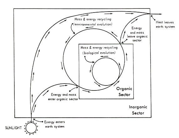
Figure 1. A general representation of mass and energy flow through the earth's surface system, with the latter envisioned as divided into two subsectors. See text for discussion.

[[p. 36]] is no progressive change in the components making up the system over time (Schrodinger, 1945; Maruyama, 1960, 1963). Under such uniformitarian conditions, when subsystems of limited lifespan reach the end of their usual terms of existence, they are replaced by like entities.

    Cross-sectional studies tend to emphasize the means through which systems maintain equilibrium under ranges of conditions imposed by external forces. In general, subsystemization is viewed in such instances as contributing to system "invariability" (Weiss, 1971). This perspective leads to a view of organismal function dominated by a "deviation-from-norm" kind of thinking; i.e., that the functions of particular biological subsystems can be stated in terms of ranges of input to, and output from, the unit (Wiener, 1949; Ashby, 1956; Conrad, 1983). To one degree or another, therefore, studies linking the state of organisms to the immediate state of their environment are implicitly applications of the theory of limiting factors (Trudinger et al., 1979).

    When the investigator wishes to study processes involving irreversible change, the cross-sectional approach depicted above proves too confining. In such work, a more critical consideration of the way intrasystem feedback controls develop becomes necessary. As Carson (1969: 76) states:

"A system may achieve equilibrium between form and process (assuming that the external variables which control the processes do not change) almost immediately in some cases; in other instances, the system may proceed so slowly towards equilibrium that an evolutionary approach is necessary to understand the nature of the system at any one point in time. In the situations where a system rapidly achieves equilibrium between form and process, an evolutionary model is unnecessary and a complete understanding of the nature of the system is furnished by a knowledge of the way in which the equilibrium pattern depends upon the external variables. An exception occurs when the outside variables themselves change through time in a systematic manner: although it is still possible to understand the nature of the system at any one point in time by references to the current state of the controlling variables, a more complete explanation is afforded by setting the system in a historical framework."

[[p. 37]] In the above passage Carson suggests two things of importance: 1) that evolutionary (irreversible) change in a system may be linked to controls set by exogenous variables, and 2) that irrespective of such change, the current state of the system can still be understood in terms of those same variables. Maruyama (1960, 1963) and Zadeh (1969) have introduced similar ideas. The notion that exogenous factors control organic evolution is not a new one, of course, but the tendency has been to dwell on the way such factors exert influences on the development of particular populations or phylogenies. In Chapter II I suggested that this strategy invariably leads to little more than the identification of correlations between adaptive responses and environment. This route will not be followed here. Instead, we will begin with the idea that the biotic sector as a whole evolves in response to constraints set by the abiotic sector. This argument will be made independently of any particulars regarding what we normally consider the "characteristics" of biological evolution (i.e., the temporal unfolding of phyletic lineages and appearance of associated adaptational innovations).

System Controls and Exchanges

    It is relatively easy to state the conditions of existence of a system in steady-state with its environment. First, thermodynamic equilibrium is maintained, a simple consequence of the law of conservation of energy. Second, it is assumed under steady-state conditions that the amount of negentropy imported to the system remains equal to the entropy generated by it (H.T. Odum, 1971; Conrad, 1983; Huggett, 1980). This constraint limits the kinds of change possible within the system to uniformitarian kinds of adjustment; i.e., to the aforementioned maintenance process [[p. 38]] characterized by replacement of "worn-out" subsystems by subsystems of like structure.

    The description of the state of a system changing in an ordered fashion through time is more complicated, since change must be explained in the face of ambient ecological equilibrium. As Huggett (1980) points out, the very word "equilibrium" implies absence of change, yet at some level of organization every system is undergoing change. The earth as a whole, for example, operates under very nearly steady-state conditions with respect to total energy throughput; nonetheless, its surface, at least, has undergone a continual process of evolution since it came into being. We must conclude from this historical fact that steady-state conditions have not actually been reached in the earth's surface system; that is, that negentropy import slightly exceeds total entropy produced. The first effect of this apparent paradox is to leave us with a problem regarding terminology. Some geomorphologists (see discussion in Huggett, 1980) have attempted to resolve this difficulty by viewing systems whose input-output balance changes only very slowly with time as being in a state of dynamic equilibrium, and this will be the solution adopted here. Thus, for purposes of cross-sectional study and depiction of the earth-level energy balance, the earth represents a steady-state system that is in dynamic equilibrium. With respect to the evolutionary development of its component subsystems, however, it is in continuous dis-equilibrium. In Carson's terms, form and process are not in equilibrium. (That they are not is all the more reason for avoiding historical models linking particular processes to particular forms, because the relationships involved are likely to be transient ones that cannot be spatially generalized.)

    We will assume for the purposes of remaining discussion, and in concert [[p. 39]] with the opinion of others (e.g., Prigogine, 1947, 1961; Wiley and Brooks, 1982; Nicolis and Prigogine, 1977; Chorley and Kennedy, 1971; Iberall, 1976) that the earth's surface constitutes a nonequilibrium system describing a movement toward steady-state energy conditions and a dynamic equilibrium material turnover state. Given this framework, a model of the dis-equilibrium attending this movement will now be used as the base for making predictions about the way organisms should be distributed in space. We need first give attention to the general evolutionary setting of the biotic sector.

    Though the emphasis here is on the evolution of the biotic sector, it is apparent that the conditions underlying change in it and the abiotic sector are mutually causal (in the sense of Maruyama, 1963): both energy and material resources move through each and back and forth from one to the other. As a result, intra-sector processes in each may be viewed as exogenous variables with respect to the operation of the other. Nonetheless, the two differ in that the abiotic sector as defined represents the only set of exogenous influences on biotic sector organization (whereas input to the abiotic sector originates in both the biotic sector and extra-system sources, especially the sun). This fact makes it easier to establish a simple causal model of biotic sector evolution. To maintain high levels of order in a living system, negentropy must be imported to it (Schrodinger, 1945; Maruyama, 1963; Kuppers, 1983). It follows from initial definitions that all such import to the biotic sector must pass through the interfaces between the latter and the abiotic sector. Across these move the resources that are necessary to the maintenance of biological activity; these have been "made available" to the biotic sector through the operation of return pathways that have evolved within the abiotic sector (e. g., [[p. 40]] biogeochemical cycles in the more obvious sense, and organismal death--which is often directly followed by ingestion by other organisms--in a less obvious sense).

    Regardless of whether the abiotic sector can "make available" the resources necessary to life, negentropy import can only be accomplished when two conditions are met: 1) when organisms capable of assimilating resources exist, and 2) when the latter are present when and where the resources are available. If we are to define a state-space involving the biotic sector and its abiotic environment, therefore, we must grant that evolution has produced organisms capable of both finding and processing the resources necessary to their individual maintenance as steady-state systems. This is taken here as given.

    A second fundamental notion is that obtaining and assimilating resources requires energy. This investment leads to an immediate net increase in entropy levels within the biotic sector as chemical energy is converted to heat. The increase is then balanced, however, by the negentropy gained (imported) as the ultimate result of assimilation of foodstuffs.

    The important thing to note in the straightforward description given above is that it suggests two different views of the meaning of the energy budget of organisms (singularly or in the collective sense). When assimilation processes are viewed in terms of the energy budget supporting them, steady-state conditions are implicitly recognized and the meaning of the energy expended cannot be extended to an evolutionary understanding. On the other hand, when the energy budget of the organism is seen as committed to spatial interaction with the elements of its environment, a more dynamic view is possible. Specifically, the energy expended by the organism can [[p. 41]] potentially be understood as contributing to change within that environment. Where its activities result in a change that ultimately leads to a net reduction in the amount of energy that need be expended to obtain and re-assimilate a given resource, it follows that evolution within the overall biotic sector has occurred: the same amount of negentropy has been imported at a lower cost in entropy production. We might thus understand biological evolution to proceed as a nonequilibrium process in which organismal activity contributes to a continually more efficient resource turnover process.

    The idea that refinement in the turnover characteristics of environmental resources is related to community development toward steady-state conditions is fundamental to the theory of ecological succession. E.P. Odum (1971: 256-257), for example, states:

    "An important trend in successional development is the closing or 'tightening' of the biogeochemical cycling of major nutrients, such as nitrogen, phosphorous, and calcium...Mature systems, as compared to developing ones, have a greater capacity to entrap and hold nutrients, for cycling within the system."

The recursive view of change expressed in the above seems at first encounter similar to the systems view of surface processes evolution being developed here. Moreover, inherent in the notion of succession is the idea that physical environmental changes have an important effect on where and when community change will occur. Nonetheless, ecological succession must be viewed as a uniformitarian process when placed within its context in system evolution in general, and probably lacks the flexibility to be applied to the study of the evolution of populations. This is most forcefully evident in the difficulties attending use of the term "climax" (E.P. Odum, 1971; Oosting, 1956; Whittaker, 1953). The ecological climax is a steady-state condition virtually by definition, a philosophical constraint that conflicts [[p. 42]] with the knowledge that population-level evolution must be proceeding even as ecological equilibrium is reached. Perhaps the best that can be done under these circumstances is to suggest that the "tightening" of resource cycles must work at two levels: one involving the short-term integration of populations into stable, self-reproducing community structures, and another involving a kind of change in organisms that leads in the long-term sense to ever more efficient climax structures. Our interest is more in the latter process, so succession will not be dealt with further here.

    The recursive nature of development of resource cycles is also treated in the literature on biogeochemical succession (note, for example, Trudinger et al., 1979; Hutchinson, 1964; Cloud, 1976; Van Valen, 1971b; Windley, 1975). The orientation of related discussions, however, tends to be similar to that concerning ecological succession. Again, this introduces a degree of inflexibility that is difficult to overcome when evolutionary explanations are sought. A more adaptable understanding can be obtained by more directly relating the turnover of resources to population-level change.

    Every organism (or population) acts as a mediator in the general turnover of resources in its encompassing environment. Obtaining resources requires an expenditure of energy, and, as suggested earlier, if there should occur from one turnover cycle to the next a general reduction in the amount of energy expended by a population to obtain a given resource, all other things remaining equal it follows that the overall system has undergone evolution (note, however, that we cannot conclude that evolution has occurred within that particular population). This will be true most fundamentally because there will have been a net reduction in the amount of entropy produced by the system over time. Before we can suggest how this idea is related to the evolution of individual populations, however, we must [[p. 43]] return for a while to discussion of biotic-abiotic sector interaction.

    Complex systems are often characterized in terms of feedback relationships. Huggett (1980: 91) describes these as follows:

"....The interplay of positive- and negative-feedback relations in a system can be subtle. Paradoxically, both types of relation can operate simultaneously to maintain the over-all stability of a system....homeostasis is that group of system-stabilizing relations which are characterized by negative feedback; homeorhesis is that group of system-stabilizing relations which are characterized by positive feedback. Homeostasis may be thought of as all those relations which act to preserve a system by keeping it in steady state during its existence. Homeorhesis may be thought of as all those relations which act to preserve not a steady state but a flow process...."

In the general system described by Figure 1, the biotic sector is characterized by the interaction of single positive and negative feedback processes. Positive feedback from the abiotic sector enters the biotic sector as a flow of (potential) energy and materials which fuels both life-sustaining and system-changing processes. How should we characterize this flow in terms of the phenomenon of adaptation? In one sense, adaptations can be viewed as homeostatic devices. Again, when the energy budget of an organism is considered in terms of its own thermodynamic equilibrium, steady-state conditions are envisioned; the structural ends to such self-maintenance may be termed adaptations. On the other hand, when its energy budget is viewed as being committed to a routine of activity that contributes to spatial interaction, the adaptational suite of the organism can be construed as serving a homeorhesic purpose. Potential nonequilibrium conditions are created when the organism returns energy and materials to the abiotic sector in amounts essentially equal to those received, but at different locations. All we need assume is that there is spatial interaction among the locations of input and output; i. e., that the organism's operation within its behavioral space contributes to a non-random [[p. 44]] change in the manner in which energy and materials are later made available again.

    The biotic sector evolution model initiated earlier can now be completed in outline by suggesting that it is the process of adaptation that signifies increasing levels of negentropy in the system; that is, that mediates evolutionary change by making possible increasingly efficient resource turnover. This leads us in the direction of spatial interaction modelling. Thus far, I have suggested that general system evolution occurs as abiotic-biotic sector equilibrium is lost, or, more precisely, as adaptation produces the means whereby organismal activity results in a net reduction in the amount of energy required to return vital resources to the same stage in a given cycle type. I have not yet specified the mechanism that actually initiates the process of adaptation that keeps the members of each population system in continuing thermodynamic equilibrium as the abiotic sector changes in response to historical inertia. This, I maintain, is movement through space and the spatial interaction that is part and parcel of that movement. A primary characteristic of living things is their ability to change location within their frame of reference. Such movement may be restricted to certain portions of a life cycle, but there is surely nothing alive which lacks this ability. Changes in location serve the immediate purpose of bringing an individual organism into physical reach of those items necessary to life maintenance; in the longer term sense, moreover, population-level locational adjustments may be viewed as acts which are necessary to/inherent in the continuation of steady-state conditions in the face of the reality of ever-changing environmental conditions. However, the steady-state approached at any cross-sectional instant can never be maintained. The particular suite of adaptations [[p. 45]] developed in response to one set of conditions will never be quite appropriate in dealing with any later conditions. The biological process representing the on-going resolution of this disequilibrium is competition; the biological result of the process is the development of new responses to the sets of conditions encountered; i.e., new adaptations.

    The above line of reasoning is not particularly remarkable and requires little further comment here. What I should like to explore in the remainder of this work is the possibility that the net direction of organismal locational adjustment on the terms presented may be predictable. If this is so and the main underlying factors can be isolated, we will then have a model which can be applied to more than just a consideration of net biotic sector evolutionary trends.

    It is relatively easy to use the ideas presented so far in this chapter to develop a model leading to the prediction of direction of range change by populations. Simply, we should expect those areas where vital resources are being returned to availability at the most ideal rates to be those toward which ranges will most likely extend. Where resources are returned at suboptimal rates (note that the term "rate" here is used to denote a pattern of return involving both spatial and temporal components) it will be necessary for organisms to evolve special adaptations (behavioral and/or morphological) enabling them to maintain thermodynamic equilibrium while functionally being "at the right place at the right time" to collect and process these resources. (A good example of this kind of adjustment is offered by the irregular conditions of water supply in deserts and the many special strategies that desert plants have invoked to ensure successful reproduction when precipitation does occur). The process of selection underpinning such change will consume both energy and time; as a result, [[p. 46]] suboptimal habitats will be occupied more slowly, all other things being equal.

    It can be argued that earlier statements being true, the above must be true as well. Were range adjustments directionally random in nature, we would expect to derive no net change in the overall state of the system--that is, evolution would not be occurring, because all instances of relative gain in system information levels would be balanced by relative losses elsewhere. Directional channelling of range change is thus the only way that consistent gains can be made.

    The focus of this discussion must now begin to change from deduction to the identification of means whereby the ideas can be tested. This will first involve relating the dynamics of population range change to the supposed spatial variation in return rate characteristics of vital resources.

Spatial Interaction and Evolution

    The most obvious spatial characteristic of a population is its distributional range. This will change through time as the population responds to various influences; in fact, distributional range is a direct correlate to the evolutionary history of a given population, since it will appear as a delimitable pattern with the initial divergence of the form and disappear with its extinction. This correlation between range and habitat has frequently been interpreted as a causal relationship. Limiting factors concepts better referred to individual-environment interaction have been used time and time again to justify the idea that species X appears limited to a certain areal distribution. Whether this extension of individual level thermodynamics to the population level is legitimate is debatable, but use [[p. 47]] of the device at least provides a reasonably straightforward portrayal of microstate dynamics. The state-space picture that emerges is of a direct coupling between a positive feedback flow (materials and energy made available to the biotic sector as a function of their transmission through the abiotic sector) and a negative feedback response (behavior and morphology).

    Recall that the steady-state recognized above is, however, a fiction in the longer-term sense. We know that the system, and its component populations, change irreversibly over time. I have already suggested how we might view this change at the level of biotic sector functions. To apply these notions to the modelling of individual population change necessitates re-assessing the notion of environmental "control." Specifically, the action of environment must be interpreted as forcing change rather than constancy. For the first step in this re-assessment we are indebted to the work of Maruyama (1963).

    Maruyama (1963) made an important contribution to General Systems Theory with his delineation of the concepts of "deviation-amplifying positive feedback" and "deviation-countering negative feedback." The following quotation from Greer-Wooten (1972: 17-18) is useful at this point:

    "The fact that the second law of thermodynamics holds for an open system plus its environment, but not for the system itself, does not appear to have been sufficiently appreciated earlier. The 'steady state' is defined by the approach of minimum entropy production, and in fact at that time entropy is maximized--subject to the conditions in which the steady state was attained. There is thus a continual tendency to the development of maximum entropy, given a certain structure and set of input and export relationships for the open system. Any changes in the environment will result in disequilibrium and the beginning of a new cycle.

    Chorley describes such developments with changed imports as the open system tending towards higher levels of organization, becoming more ordered and heterogeneous. Such changes appear to be contrary to the second law, but Maruyama accounted for them by [[p. 48]] deriving important notions to describe open system change in general. If the exchanges of the system with its environment do not change markedly, then entropy production continues to be maximized up to the steady state. Such imports have been labelled negative entropy (or negentropy) and are also called 'information' and 'order.' However, the reactions of the system components to imports from the environment are also important in describing system change. Such system 'feedbacks' can be of two types: negative feedbacks (deviation-countering processes) maintain equilibrium situations, conditions that Maruyama called 'morphostasis;' in comparison, positive feedbacks (deviation-amplifying) influence system change, whether it be towards greater or less order....

    One important conclusion that can be drawn from the discussion above is that in analyzing the dynamics of systems, the researcher should place more emphasis on flows (of energy, materials or information) between components of the system, and the system and its environment, than on changed attributes of the elements."

    In the above passage there is a point made that is especially important to the present discussion. This is the notion that a system may respond to imports from its environment through either deviation-countering or deviation-amplifying processes. It has already been suggested that adaptation can be viewed as a deviation-countering process; accepting this idea allows us to maintain the classical physio-ecological truism that an organism must be adapted to the conditions imposed upon it by its environment to persist there. As earlier stated, however, range change and the history of the evolution of adaptations must be interpreted as indicative of a system that is not in equilibrium; i.e., that a deviation-amplifying process is also in operation., The ongoing development of new adaptations can be viewed as no more than a continuous change in: 1) the means by which equilibrium conditions are approached (homeostatic view); or 2) the potential for effecting change (homeorhetic view). The process of change itself is the movement of the overall biotic sector away from equilibrium and in the direction of higher levels of order, and in this adaptation plays only an indirect role.

    [[p. 49]] If we accept the above a number of important results fall out. Most importantly, we are led to question (as have Gould and Lewontin, 1979) whether evolutionary change is best viewed in terms of adaptational structures. Neither the homeostatic nor the homeorhetic view of the function of adaptations casts the latter as actual evolution; rather, at most they seem to represent a physical correlate to the interaction state that more aptly describes it (a view that can be extended to the process of adaptation as well: Wiebes (1982: 243) has appropriatedly dubbed this "the historical narrative of evolution"). This interaction state is based in spatial relationships; that is, in the way the spatial structure of the biotic and abiotic sectors influences the turnover characteristics of resources. To a certain extent one might argue that the implied relationship of adaptation and spatial interaction to evolution reduces to a "chicken or egg" circularity, but there are important reasons why this should not be considered the end of the matter:

    1) To begin with, the new causal relationship posed between adaptation and spatial interaction lends its way to both state-space and process interpretations. In this understanding, Carson's (1969) "outside variables" (abiotic sector provision of vital resources) can be linked to a system response that may be stated as either ecological state-maintenance (equilibrium) or evolutionary dynamism (disequilibrium). As part of a discussion of Wiley and Brooks (1982) Whitten (1983: 442) has recently remarked:

"....internal ordering depends on a system's ability to export entropy to its environment .... The virtue of the thermodynamic approach to evolution is its ability to connect life ecologically to the rest of nature through shared matter and energy flows; denying the ecological component of evolution, or the influence of ecology on development, badly weakens (their) thermodynamic base."

[[p. 50]] Wiley and Brooks (1982) introduced a nonequilibrium approach to evolution that has been strongly criticized on a number of counts (especially note Lovtrup, 1983; Bookstein, 1983). Whitten (1983) is of the opinion that, though the model itself is "quite flawed" (p. 438), its "spirit" is welcome. Here, I present a model of evolutionary change which, though "in the spirit of" the Wiley and Brooks effort, differs from it by stating nonequilibrium conditions in spatial terms rather than biological ones. This causal structure provides a convenient basis for testing possible models involving evolutionary change, since as discussed in Chapter II one of the greatest strengths of the ecological approach to biogeography lies in its methods of dealing with identifiable constraints on range change.

    2) Moreover, this understanding of the entirely separable--but still complementary--roles of spatial interaction (and its implicit result: distributional change) and adaptation solves outright the philosophical dilemma attending the view that evolution involves a process (adaptation) that yields structures (adaptation) of non-independent definition (Brookfield, 1982; Ghiselin, 1966; Grene, 1971; Gould and Lewontin, 1979). As Lewontin (1984: 237-238) has put it, "The process is adaptation and the end result is the state of being adapted...The problem is how species can be at all times both adapting and adapted." When evolution is understood as the disequilibrium characteristics of biotic sector/abiotic sector spatial interaction (and not "the process of adaptation"), the homeostatic, "ecological," role of adaptation can be accented to provide a straightforward causal picture devoid of circularity and attending logical difficulties. In this view, adaptations are regarded simply as the structural attributes that mediate energy degradation, or that, as Wicken (1983: 440) puts it, "provide a means by which potential energy can be [[p. 51]] converted to thermal entropy and released to space." The problem that Wicken (1983), Wiley and Brooks (1982), Lovtrup (1983), and Bookstein (1983) have not been able to resolve is precisely how progressively greater amounts of this just-referred-to potential energy are converted over time; i.e., why evolution and not equilibrium? Wicken (1983; 440) edges nearest to an answer by suggesting that it is natural selection "which selectively preserves certain sequences (i.e., adaptations) while rejecting others." Again, however, a label has been attached here to a spatial interaction process that is not specified as such, and it thus remains a fuzzy concept.

    3) Further, re-interpreting evolution as a spatial interaction process provides a response to the complaint that the study of the "evolution" of adaptations (i.e., phylogenetic studies) reduces to narrative. It still must be accepted that particular adaptations arise as responses to one-of-a-kind combinations of environmental and biological circumstances. It must also be accepted that this understanding resists any ordered interpretation beyond the identification of when and where each arose (and the sequencing of this information with all other such information). But when the homeorhetic function of adaptations is recognized, these criticisms are rendered moot. When adaptations are viewed as structures underpinning spatial interaction, they can also be implicitly understood to promote system "flow" toward steady-state conditions. Whereas the homeostatic function of adaptations is simply to mediate the conversion of potential energy to thermal entropy (per discussion in the last paragraph), their homeorhetic function may be viewed as the mediation of spatial interaction. As resource re-cycling capabilities of the system tighten as a general function of the latter, less thermal entropy needs be generated per potential energy imported (the result being system evolution). We therefore [[p. 52]] needn't think of evolution as leading to the unique structures we call adaptations, but instead to standing interaction processes interpretable on normative grounds: in the biological sense, for example, as competition/natural selection, and in the spatial sense as distribution patterns. In this view, it is more the properties of spatial interaction that evolve than the organisms themselves.

    4) Lastly, the causal structure posed between spatial interaction and adaptations provides a framework within which long-standing issues in evolutionary theory might be examined in new ways. An example is provided by the "saltationist-incrementalist" debate; that is, whether evolution proceeds in sudden starts and stops or as a gradualistic process (see Eldredge and Gould (1972) for representative discussion). This discussion must be separated into two components when examined in the light of ideas set out here. There is first the one that has existed all along--that the fossil record does not suggest a gradualistic kind of evolutionary progression despite the fact that this is what classical (as well as Neo-Darwinian) selection theory logically demands. But the fossil record can only document changes in structure; i.e., in mode of adaptation. I have just argued that bodily form/behavior can be held to represent either the results of evolution, or a kind of potential for evolution, but not the interaction process constituting evolution itself. Importantly, regardless of whether saltation can describe the manner of sequential unfolding of adaptive assemblages, it may or may not describe the way changes in the spatial interaction structure of the biotic sector take place. This realization helps us to identify a fundamental problem in the way saltationist/gradualist discussions have developed. The gradualism point of view (e.g., as held by Darwin, Mayr, Simpson, and Wallace) is [[p. 53]] fundamentally an externalist's approach to evolution; through it natural selection becomes largely a function of environment (whether the latter be specified in physical or biological terms). Those who take an incrementalist stance, on the other hand, implicitly fall into an internalist's mode of thinking: that evolution is regulated by potentials and constraints that are acted upon by the environment (note the arguments of Gould and Lewontin, 1979; Gould and Vrba, 1982). It is pointless to ask which of these is the actual mode of evolution. While the nature of spatial interaction changes with time, this is almost certainly a gradualistic process, since it must be a function of a collective biotic sector change process mediated by changes in the abiotic sector. It has been the mistake of the gradualists to synonymize evolution with observable changes in form of organisms over time; this view leads to the "adaptation yields adaptation" circularity philosophically, and to the empirical contradictions of the fossil record. Arguments denying gradualism, on the other hand, are equally short-sighted. It can hardly be believed that environment-originated selection factors do not have important influence on the way characters are selected, regardless of whether population-specific constraints are also involved, or, for that matter, whether the fossil record can be proven to indicate saltational patterns of change. What is actually being "selected" is not a suite of adaptations, but instead a means of turning over material resources. In short, the central issue to be resolved is exactly how gradualistic change in spatial interaction patterns yields saltation in the development of individual phylogenies, and not whether one or the other is "correct." Despite the fact that his analysis focuses on internal factors in evolution, Waesberghe (1982: 26) comes to similar conclusions: "To an alternative model evolution is the saltatory [[p. 54]] origin of new taxa, prepared by a gradually improved ecosystem of interdependent external and internal factors."

    (For the sake of internal consistency it should be pointed out that the comments of the last paragraphs apply equally well to a consideration of abiotic sector evolution. It is the erosion and transport of rock materials from various locations and their eventual deposition together in new ones that leads to the production of ever-more diversely constituted rock units. Orogeny in this sense is a process directly analogous to adaptation; in both cases the structural outcomes: 1) are time- and place-specific; 2) are novel and irreversible; 3) are impermanent; 4) are products of local conditions ultimately set by the unfolding of larger scale/longer term geological/climatological processes; and 5) fall out regardless of the particulars of history and composition (i.e., rock type and organism type) associated with them.)

The view held here of the dynamic interrelationships among distributional changes in populations, their adaptive capabilities, and environmental input might be stated in slightly more general terms at this point with the aid of the following quotation from Boulding (1956: 13):

    "Another phenomenon of almost universal significance for all disciplines is that of the interaction of an "individual" of some kind with its environment....each of these individuals exhibits 'behavior,' action, or change, and this behavior is considered to be related in some way to the environment of the individual--that is, with some other individuals with which it comes into contact or into some relationship....The 'behavior' of each individual is 'explained'....by certain principles of equilibrium or homeostasis according to which certain 'states' of the individual are 'preferred.' Behavior is described in terms of the restoration of these preferred states when they are disturbed by changes in the environment."

In the present context the "individual" is a population, and "behavior" is synonymously range (spatial) change and adaptation. The latter two are [[p. 55]] viewed here as complementary understandings of a single process in which each population contributes to a slow system-wide progression toward steady-state conditions. In this work I concentrate on the spatial interpretation of the "behavior" concept portrayed above. This allows us to understand the "preferred states" of organisms/populations as being evolutionarily transient and individually unique in a biological sense (adaptation), yet still subject to normative interpretation (as distribution patterns belieing non-random states of spatial interaction among populations and their environment).

Spatial Interaction in the Community Context

    We have now approached a means through which to translate an aspatial and cross-sectional understanding of abiotic-biotic relationships (e.g., the first interpretation given of Figure 1) into a spatial and process-oriented version of the same that can be related to population-level change. There is one more matter to consider in this chapter before we can turn to the formal modelling considerations leading to hypothesis tests, however. This is also the most difficult to approach, for we must now bring together all that has preceded into a single comprehensive view that is conducive to such modelling. To accomplish this, we must consider the relationship of range change, as interpreted through the present approach, to changing community structure.

    While range change is usually examined from the perspective of within-population processes (as in Parsons, 1983; Van Valen, 1971a), it is clear that it does not take place in the larger sense in a void: changes in population distribution characteristics also reflect the constraints set by local community organization properties (Brown, 1983, Chapter Four). There [[p. 56]] is, moreover, a real advantage to looking at zoogeographic change patterns from the community level: flexibility. From an analytical standpoint (and per earlier discussion), it is difficult to view a species population as other than an ecological or a historical entity, because the species is a relatively individual and "irreversible" entity in both space and time (Ruse, 1973; Ghiselin, 1980. The historical element implicit in the notion of species is its genetic relation to other species (that is, its relative position in the life hierarchy), not to the history of the ecological system continuously sustaining it. Little information regarding the location of the particular community in which an organism happens to find itself is stored in the form of adaptations (one immediate reason why physiological ecologists have had little luck with evolutionary modelling). Communities, on the other hand, are neither rigidly delimited--or even, perhaps, delimitable--in space and time nor express much of anything about their "genetic" relationship to communities elsewhere. Nonetheless, like species, their characteristics can easily be linked to ambient environmental conditions, and they do exhibit a historical side: the pattern, over time, of assimilation of species populations into them.

    This is an important association. It affords a means through which historical process can be viewed in terms of spatial interaction instead of the irreversible evolutionary outcomes that are the product of phylogenies: both subtraction and addition of forms characterize change in a community through time. With the switch to the spatial interaction approach emerges the possibility of normative modelling of distribution patterns. To begin with, all populations are members of communities ipso facto and contribute to the non-population-specific resource turnover processes mediated by community structures. The important consideration, however, is whether the [[p. 57]] reverse can be shown as likely: that turnover characteristics in space and time of some one (or more) vital resource lead to the assimilation characteristics in space and time of populations into communities. Biologically, these "characteristics of assimilation" will include a bewildering array of adaptive changes and strategies dependent on population-specific histories, and will be difficult to link, across all populations, to individual abiotic sector forcing functions. The spatial character of assimilation, however, will be directly evident in changing distribution patterns, which might be interpreted more easily: for example, as a function of spatial variation in one or more fundamentally vital abiotic sector-mediated variable.

    Supposing that it is useless to attempt a definition of community grounded in the evolutionary histories of the species populations making up communities, there can likewise be no prior meaning attached to the specific suite of phenotypic expressions associated with them. This is not to say that general classes of adaptational strategies (adaptation to extremes of cold, heat, moisture, etc.) cannot be linked to particular kinds of habitats or community structures, but instead to again point out that the genetic means to such ends are in a historical/phylogenetic sense idiosyncratic; that is, taxon-specific (a re-statement of the individualistic hypothesis). Our only other option, it seems, is to believe that particular lineages and strategy types come together necessarily to generate the community characteristics we witness, a teleological viewpoint that can be reconciled neither with the geographic understanding that interaction in space is stochastic nor with empirical evidence presented by supporters of the individualistic hypothesis. Neither does it seem reasonable to argue that the vagaries of change in the physical environment [[p. 58]] can somehow be directly foreseen by organisms, unless we are willing to accept a Creationist stance.

    A conservative way to treat community assimilation processes is thus to start with the hypothesis that communities are accidental structures that evolve as a simple function of the particular populations that happen to arrive and become integrated into them. This view, in fact, is little different from the current framing of "community" as a "concept" rather than a prior reality (see related discussions in Gleason, 1926, 1939; Cain, 1947; Saarinen, 1982; Whittaker, 1962, 1973; McIntosh, 1967; Pielou, 1974). The individualistic view is well summed up by Whittaker (1973: 327):

"Species are distributed 'individualistically,' each according to its own way of relating to environment....Species do not fit naturally into groupings that correspond to community-types and are discontinuous with other such groupings....Community-types are not natural but arbitrary units in the sense that their extensional definitions are strongly influenced if not wholly determined by phytosociologists' choices of the characteristics by which communities are to be classified....further....not only species but also groupings of species....show relative independence of one another, and may be differently combined into particular communities."

It is thus argued that, in terms of those populations coming together, community structure will develop as a non-predetermined function of their collective adaptive flexibility. This point of view seemingly casts long-term community-level change as a kind of chance drift phenomenon analogous to the one now thought to take place at the genetic level (Kimura, 1983a, 1983b; King and Jukes, 1969). Were communities entirely self-contained, we might be able to accept this notion as a means of depicting the associations that emerge among community members; clearly, however, communities are not isolated systems. Communities can be viewed as geographically-limited portions of the biotic sector. Like the biotic sector in general, they depend on the abiotic sector to provide the means of [[p. 59]] turnover of resources. This exogenous influence must effect controls on their operation and development (H.T. Odum, 1967, 1971). Attention must be drawn to how this exogenous influence might be implemented.

    One of the most common ways to relate exogenous controls to the character of community interaction patterns is through the concepts of density dependence and density independence. The former involve selection factors whose effects on population vary with population density (Smith, 1961; Lack, 1954; Nicholson, 1957); the latter, factors whose effects do not, and that therefore are proportional to density (Andrewartha and Birch, 1954; Davidson and Andrewartha, 1948). Climatic influences on selection are usually considered to be of the density-independent type, whereas more strictly biological interactions such as competition, predation, and disease tend to be density-dependent in their selective capacity.

    The development of these concepts (and the related r- and K-selection continuum notion: see MacArthur and Wilson, 1967; Van Valen, 1971a) has implicitly forced evolutionary ecologists into thinking that selection controls fall into classes only one of whose elements are exogenous to the community interaction structure. Although this approach makes it easier to appreciate the demographics of individual populations, it is less effective in suggesting how change in the recursive processes of resource turnover--and thus general system evolution--develops between the biotic and abiotic sectors. A simplification relevant to such understanding should now be noted. In the resource cycle model developed here (i.e., Figure 1), there is no differentiation between density-dependent and density-independent types of selection processes, because all exogenous influences on biotic sector elements are exerted by the abiotic sector. As defined earlier, the biotic sector is comprised of organismal "islands;" all [[p. 60]] imports/exports to/from each organismal unit involve crossings of the biotic-abiotic interface. The importance of emphasizing this feature of the present model now will become apparent shortly.

    Recognition of the fact that communities can be de-stabilized under the influence of exogenous forces has led to much study. There appear to be two major accents in the relevant literature: the more abstract notions of community stability and resilience, and the characterization of stressed ecosystems. The first subject cannot be satisfactorily reviewed here without pulling us too far off the track (see Holling, 1969; 1973; Margalef, 1969; Lewontin, 1969; May, 1973). Since the concept of stress is directly relevant to present purposes, however, the following extract from Franz (1981: 50) is reprinted (minus original references to literature) in an effort to briefly review how it has been historically treated:

"Stress as Cause

According to this approach, stress acts as an independent variable, external to the organism, being a stimulus or input which causes strain. This approach depends heavily on analogy with Hooke's law....According to Levitt, stress is any environmental factor which is potentially unfavourable. The evolutionary response of organisms has been selection for avoidance or tolerance of the strain.

Stress as Effect

According to this approach, stress acts as a dependent variable, internal to the organism, being a response or output which is caused by some factor that is usually identified as the stressor. One of the best-known formulations of this approach is that of Hans Selye. His autobiographical account of its development emphasizes the notion that stress is the response of an animal to an external stressor. Furthermore, it is claimed that the response is physiologically non-specific and does not depend on the nature of the stressor. The stress response represents a universal pattern of defence, a mechanism to preserve the animal's integrity....

    The predominant formulation of stress as effect is based upon performance. An organism is in a state of stress when some measure of its performance falls below par. This formulation can [[p. 61]] be traced to Liebig's law of the minimum or to Shelford's extension of it, the law of toleration. This tradition is basic to much of the experimental work in comparative animal physiology and agronomy. It recognizes that stress can be induced by environmental factors which are either above or below the optimum range. As no species encounters in any given habitat the optimum conditions for all of its functions, performance can be enhanced, as well as diminished, by manipulation of the environment. E.P. Odum et al. have referred to this effect as the subsidy-stress gradient. This effect is not confined to enrichment alone; impoverishment results in a subsidy when an environmental factor in excess is restored to the optimum range...."

Franz's discussion continues in a direction that is also of interest here: stress as both cause and effect. To complete our model here, we need to identify a way in which the rate/pattern of provision of some vital resource(s) causes an influence on the development and operation of community structure that forces a deviation from the drift-like conditions imagined under a strict interpretation of the individualistic hypothesis. This influence, to be referred to as "stress" from here on, will be expected on the basis of earlier remarks to be linked to two kinds of complementary results: 1) a biological result, manifest at various organizational levels as community, population/demographic, and adaptational (morphological, physiological, and behavioral) structures and changes in same over time; and 2) a spatial result, manifest as distributional patterns and the way these change over time. Franz proceeds to comments pertaining largely to the first subject; we shall continue our attempt to develop ideas related to the second.

    Let us first imagine a hypothetical vital resource that cycles through both the biotic and abiotic sectors but is essentially ubiquitous in time and space (atmospheric oxygen represents a fair approximation). Such a resource can represent neither a selection factor nor an influence on distribution, as it will not be competed for and will prescribe no patterns [[p. 62]] of interaction with elements of the environment. On the other hand, a vital resource that is only available in potentially useful amounts part of the time and/or in some places is by definition limited and can be understood to exert the latter kinds of influences. The biological results produced by the operation of such influences form a greater part of the biological literature and need not be dwelled on here. The results, expressed in terms of spatial interaction, however, are central to the discussion.

    It is apparent that any resource that is vital to all forms of life but is only available part of the time and/or in some places will dictate certain spatial strategies of existence on the part of living things. Specifically, they will need to apportion a significant part of their total energy budget to the development and operation of means of being "in the right place at the right time" to obtain and conserve the resource. This directed behavior, whether active or passive, will lead to the development of non-random movements through time and space (for sedentary organisms the patterns will devolve as spatially-varying rates of successes and failures of individuals over time). I interpret this deviation from random movement in time and space to represent a direct mapping of the stress upon the system. The greater the stress (i.e., the more discontinuous the rate and spatial patterns of provision of the vital resource), the more non-random the movement we should expect.

    Such non-random patterns of direct interaction between the biotic sector and the abiotic sector will of necessity extend to the pattern of interaction among organisms. An obvious example is the well-known fact that in times of drought, carnivores often hunt near the waterholes their prey frequent. Commensual and parasitic relationships provide another, as do the various kinds of mimicry and protective coloration devices.

    [[p. 63]] It should be understood that the regimentation of spatial interaction patterns in communities may be equally extreme in very different kinds of environments, though differing in specific characteristics of non-randomness. We find, for example, equally unusual adaptations in desert and tropical rainforest organisms. It may be complained at this point that there is, however, a considerable difference in the kinds of selection regimes leading to the types of specialization associated with each habitat. The evolution of desert lifestyles seems to be dominated by physical environment constraints (Andrewartha and Birch, 1954; Cloudsley-Thompson, 1964), whereas the adaptations of tropical rainforest forms usually seem to be more biologically-dictated (involving the finer niche partitioning (MacArthur, 1972; Klopfer and MacArthur, 1960) associated with, for example, mimicry, mutualism, parasitism, etc.). This criticism, however, is irrelevant to present arguments. All that is assumed here is that the degree of ordering of spatial interaction can be the same under such differing conditions of habitat. There is no reason to believe that this cannot be so, as it is known that very different ordering processes can produce non-identical structural results of equally high information content (Lenz, 1977; Getis and Boots, 1978; Shannon and Weaver, 1949). The division of influences on community interaction patterns into density-independent and density-dependent types tends to implicitly conceal this notion; attention is drawn to the results of the adaptation process (i.e., adaptations) rather than the spatial interaction process sustaining adaptation. The new understanding is consistent with earlier arguments regarding the relative roles of adaptation and spatial interaction in the evolutionary process. I do not deny the relevance of thinking in terms of density-dependence and density-independence as means of dealing with particular kinds of ecological [[p. 64]] problems; the point is, however, that this separation of concepts is not productive when it comes to modelling spatial interaction as a function of the influence of exogenous factors.

    (Note, moreover, that the spatial interaction approach advocated here can easily be applied to an understanding of the results of different kinds of selection regimes. Inasmuch as adaptations are portrayed through this view as correlates to the "geometry," as it were, of spatial interaction, wherever the exogenous conditions specifying the form of that geometry are similar, we should expect similar suites of adaptations to exist. This makes the interpretation of large-scale convergent/parallel evolution of the type studied in Mooney (1977), for example, relatively straightforward.)

    Given the spatial version of the community interaction matrix (Levins, 1968) described above the following scenario relating range change, exogenous variables, and community structure can be posed. As a direct result of degree of nonoptimality of rate and magnitude of provision of vital resources through the abiotic sector, a given community interaction matrix will develop as a non-random pattern of (spatial) interaction among organisms (and between organisms and their environment). The greater the exogenous stress involved, the greater will be the degree of spatial ordering of populations involved. The degree of stress and resulting nature of the community interaction matrix will also affect rates of in-dispersal of populations, since the latter will have to evolve behavioral/morphological structures allowing them to take part in the particular pattern of spatial interaction dictated by that stress. Where the stress is high, ordering will be great, and penetration of the structure by new populations will be more difficult because more selection will be necessary to produce the characters necessary to fitting into that order. [[p. 65]] Thus, rate of assimilation of populations into a given community will be a function of the degree of stress imposed upon the latter.

    The deductive argument for the nature of the constraints on the community assimilation process can be strengthened by appealing to an argument analogous--and perhaps homologous--to that used by proponents of the neutralist view of evolution (King and Jukes, 1969; Kimura, 1968, 1983a, 1983b). As defined by Kimura (1983a: 208), the neutral theory "asserts that the great majority of evolutionary changes at the molecular level are caused not by Darwinian selection but by random fixation of selectively neutral or nearly neutral mutants in the species." The theory further states that under such circumstances, random drift will set in with respect to relative allelic frequencies, "so that most polymorphic alleles are maintained in the species by the balance between mutational input and random extinction (or fixation)" (Kimura, 1983a: 208). With respect to community evolution, we might expect a similar process involving the assimilation of populations to take place. Where there is no exogenous control (again, where there are optimum rates of resource provision), the addition of populations might be expected to occur under a simple drift-like regime progressing toward steady-state conditions and entropy maximization. With such constraints added, however, an increasingly ordered regime of selection will be sponsored in which alleles with particular adaptive potential are selected for: the potential to take part in the degree of non-random interaction specified by the external stress.

    The degree to which community function and change operates under externally-originated stress is potentially a measureable quantity (see Barrett and Rosenberg, 1981). Moreover, in theory it should be possible to identify how this degree of stress to community development varies over [[p. 66]] geographical space. Again, if community structure otherwise develops as the random situational integration of populations (the individualistic hypothesis), it can be adduced that for any given population initially entering into that structure (through dispersal), the ease with which it will do so will be due to the degree of constraint on community drift. This is a testable hypothesis, because it suggests that direction of dispersal will tend to be toward those places that are least stressed, a proposition that can be subjected to various kinds of analysis of the pattern characteristics of actual organismal distributional ranges. In Chapter IV a model is developed that can be used to aid such efforts.

[[p. 67]] IV. SPATIAL INTERACTION AND RANGE CHANGE: AN INNOVATION DIFFUSION MODEL

Innovation Diffusion Models

    The main goal of this chapter is to develop a model of range change set within a generally accepted framework of innovation diffusion and adoption. Attention is given to the concept of innovation diffusion per se, the relation between innovation diffusion and adoption in the present context, and the formulation of an operational structure consistent with present purposes that can be used to promote hypotheses and support empirical study.

    Whereas the last chapter was devoted to the development of a general viewpoint, the present one will be concerned with the development of a model of the same relationships more conducive to analytical application. Our fundamental problem is to derive a system which: 1) is flexible enough to apply to both state-space and process interpretations of diversity characteristics; and 2) is not philosophically restrictive. The first constraint needs little further comment; our wish is to be able to view organismal distribution as being both the product of a historical process and immediate ecological controls. Philosophically, the difficulty lies in avoiding the error of developing a model which imposes a non-recursive biological or environmental determinism upon the frame of reference considered. Our model should explicitly seek a resolution between biotic and abiotic sector function that can be stated in distributional terms; this is possible only if the biotic and abiotic sectors are viewed as jointly contributing to that resolution. Again, this is not possible when we start with a prior evolutionary or environmental determinism argument, because we [[p. 68]] are falling prey to the fallacy described in Chapter II of thinking that the open system nature of evolution at a location can be fully described in those terms (Craw (1984) poses a similar argument).

    The spatial interaction approach that has been adopted here is sensitive to this philosophical problem. The coupled relationship between the abiotic and biotic sectors identified can be used to make predictions about both: 1) the probable distributional characteristics of organisms under given conditions, and 2) the complementary kinds of selection regimes that should be functioning under those same conditions. Following earlier-stated goals, we have developed a model of recursive biotic/abiotic sector interaction that is conducive to both ecological and evolutionary understandings of the meaning of distribution. The model focuses on the role spatial interaction has in evolution. We must now develop this understanding more formally.

    The spatial model used here as the device through which to base an understanding of range change in organisms is innovation diffusion and adoption. This has not to my knowledge been used in the past as a means of modelling systems operating under dynamic equilibrium conditions, but there is really no incompatibility involved. At the individual population level, innovation diffusion (in the form of range change) can be viewed as leading to some distributional outcome through which the population maximizes its contribution to system change (through its particular part in defining the spatial interaction structure of the system). At the earth system level, it can simply be viewed as the mechanism whereby steady-state thermodynamics are maintained at any given time regardless of general evolutionary trends.

    Katz et al. (1963) have defined the process of diffusion of innovation as: 1) the acceptance, 2) over time, 3) of some specific item, idea or [[p. 69]] practice, 4) by individuals, groups or other adopting units; linked to: 5) specific channels of communication, 6) a social structure, and 7) a given system of values, or culture. While this definition explicitly links innovation diffusion to human societies, close analogs to the relationships involved can be seen in the study of more strictly biological processes. For example, Anderson et al. (1962: 19) have listed the six factors involved in the infectious disease process as: 1) a causative or etiological agent; 2) a reservoir or source of the causative agent; 3) a mode of escape from the reservoir; 4) a mode of transmission from the reservoir to the potential new host; 5) a mode of entry into the new host; and 6) a susceptible host. Researchers have not failed to notice the obvious resemblance between the innovation diffusion and epidemiological perspectives, and many cross-fertilizations of approach have occurred (see discussion by Brown, 1968, 1981; Rogers, 1983). It can be suggested, in fact, that the phenomena of innovation diffusion and adoption are of such general nature as to be largely independent of context (a theme expanded on in Smith, forthcoming). It takes very little stretching of the Katz et al. view to simply cast innovation, innovation diffusion, and innovation adoption as the appearance of something that did not exist before and its subsequent integration into, and persistence within, a pre-existing system structure. A biogeographical version of the Katz et al. definition reads very easily: "Population diffusion and integration may be characterized as: 1) the introduction and integration, 2) over time and space, 3) of a population of organisms, 4) into a complex niche space; linked to: 5) specific channels of communication (geological/climatological/ecological/geographical corridors/gradients facilitating the indispersal and integration of the population), 6) an already functioning biological system resident at that location, and 7) [[p. 70]] given characteristics of stability and resilience of that biological system." A brief expansion of these concepts follows.

    "Colonization" is a term that is reflexive in the sense that implicit in it is the notion of a frame of reference within which the introduction and subsequent integration of a population can take place. In this sense, therefore, colonization involves the community at a given location "adopting" into its structure an innovation; that is, a new population. It is straightforward that this event must take place over time and space, and must involve a population (of reproducing individuals) whose presence in the system will in some way complement niche interrelationships among the forms already present there. The "channels of communication" link may seem initially a bit more difficult to translate into biological terms, but is possible if we accept that adoption in the biological sense must be a matter of immediate (in the literal sense of the term) interactions. The "channels of communication" involved must therefore be physical links between locations sponsoring movement of the elements (individuals) of the innovation (population), which will be facilitated or retarded in turn by physical enhancements of, or constraints on, such movement. There must, finally, be an existing community structure within which to fit, with the characteristics of the introduction event being relatable to that community's properties of internal order; for example, its stability and resilience (Margalef, 1969; Holling, 1969, 1973; Whittaker, 1973).

    Despite the ease of translation evidenced above, to my knowledge the innovation diffusion approach has never been deliberately applied in a specifically biogeographical context. The closest approximation to such seemingly is the MacArthur and Wilson model detailing the evolution of equilibrium faunal dynamics under insular conditions, but there is no [[p. 71]] evidence that this is a derivative of the innovation diffusion and adoption mode of thinking. Although both models treat processes relevant to the spatial flow of information and/or objects, they differ in their level of focus. The MacArthur and Wilson model specifies the pattern of evolution of faunas, concerning itself relatively little with individual populations. The study of innovations, on the other hand, is "population"-oriented, concerning itself equally with the characteristics of the "population" that is diffusing and the "population" that is adopting (Brown, 1981; Rogers, 1983). The latter framework is thus arguably a somewhat more flexible one. This is important in the treatment of continental faunal changes. Whereas equilibrium conditions in the insular situation are envisioned as maintained through the balance of largely random instances of local extinctions and colonizations (MacArthur and Wilson, 1967), continental populations are larger, ostensibly less transient, and have distribution patterns that presumably respond to perturbation in more complicated ways. When our focus of attention can be placed equally on population and frame of reference, it becomes easier to understand such responses; thus the attraction to diffusion modelling here.

    The geographical approach to the study of innovation diffusion has been most significantly developed by Hägerstrand (1952, 1965, 1967). A good review of relevant considerations has been given by Brown (1981); for the present, we shall be concerned briefly only with Hägerstrand's methodological framework, which makes use of Monte Carlo simulation techniques. To simulate the diffusion process, Hägerstrand starts by creating a grid of contiguous cells within the center cell of which an innovation is supposed to occur at a given point in time. Its pattern of spread to (and "adoption" within) other cells then becomes a function of [[p. 72]] what is termed the "mean information field" (MIF) associated with the grid. The MIF is created by assigning probability-of-adoption values to all cells (with the sum of probabilities equalling 1.0), in the simplest case through the use of a distance-decay function which specifies smaller and smaller probabilities of adoption at further and further distances from the center cell. As the simulation proceeds, therefore, cells closest to the center cell tend to become those to first adopt the innovation, with cells further away lagging behind. The result is a constrained, but still stochastic, diffusion episode.

    The Hägerstrand approach is meant to apply to situations in which innovation diffusion is possible across spatial gaps in the areal domain involved (for example, as a response to advertising via the electronic media). This obviously does not occur in the biological context with any great regularity (except, of course, in a certain sense with respect to islands). Nonetheless, the concept of the MIF can function in the present context as long as we restrict its applicable domain to the immediate neighbors of any given cell. The real problem that arises, however, is that we wish to look at the constraints on organismal diffusion at any given location (in a given "cell") as imposing an influence not only on the direction of further diffusion, but also on its rate, and the cell-by-cell approach makes this relatively difficult if we begin the diffusion from a point. Nonetheless, we need this feature, since we have already argued that spatial variation in the quality of the positive feedback signal emanating from the environment ultimately drives rates of range change. Two solutions are possible: a more complicated simulation model, or abandoning simulation approaches altogether in favor of deterministic modelling. In this study, the latter route is followed. Characteristics of distributional patterns [[p. 73]] are thus viewed as dependent variables, with the relevant influences on such emerging as independent variables. As suggested earlier, the effect is one of identifying the causal forces responsible for a kind of standing-wave pattern. This approach permits hypothesis testing, and also serves to identify patterns that later can be independently tested through simulation. As we shall see, however, we must be careful about the types of patterns we wish to identify using the deterministic modelling route.

Range Change Modelled as Innovation Diffusion

    A convenient way to describe flow interactions over space and time has been described to me by J. Huff (pers. commun.) as:

where I_ij()is the interaction (flow) between locations i and j over time period t, and z() is some set of exogenously-specified variables evaluated over the same time period t. Given comments in Chapter III concerning the complementarity of state space interpretations of distribution and adaptation, this understanding may be adapted to the present situation in the following manner. As describing material flow between environment and population and the relationship of this interaction to range change, I_ij() stands as both : 1) change (extension or contraction) of limits of range of a population from point i to point j along a linear transect along which exists a continuous sequence of the influencing set of values z(); and 2) the degree of irreversible change in the gene pool of the population concomitant with that same range limits change from point i to point j. There is a price to pay for structural change: specialization. It is a proposition here that the rate of this specialization process is a function [[p. 74]] of the exogenously-defined environmental constraints z(), which vary over space, and a factor specific to a given population, K, which does not, and that might be termed its "adaptive potential."

    To describe a given event of range extension between points i and j, therefore, we need to consider the influence of the following factors. There is first the population-specific parameter K, which gives us in general terms the potential of dispersal of the species; i.e., how rapidly it can diffuse into accessible habitats. (This conceptualization may be compared to Wallace's (1866) observations regarding the correlation between extent of range of a population and degree of variability among its individuals.) K is independent of particular locational parameters and thus enters into the consideration of range change as a parameter controlling rate only, which varies from species to species. The set of factors z() influence range change in two ways. First, where level of exogenous influence is great, rate of range change will be slower (because the population involved will be attempting a diffusion process across the more specialized kind of community structure dictated by those conditions). Second, where the level of influence varies greatly between i and j, rate of range change will be slower (because more intense selection will be necessary to adapt the organisms to the spatially-changing conditions they are encountering). These factors add up to a "certain amount of range expansion at a certain adaptational cost" interpretation of I_ij() for a particular set of conditions extending over time and space.

    The areal distribution of z()'s in the real world will be designated a "stress field." The resulting topography is a direct mapping of spatial variation in the degree to which the physical environment-mediated positive feedback signal experiences loss in potential information content before [[p. 75]] reaching the biotic sector. This concept can easily be related to the MIF of innovation diffusion studies. The latter weights the likelihood of "adoption" by a given cell; the former, the rate at which range change is likely to occur in different directions. According to this understanding, we are likely to find greatest rates of range change; 1) where stress is low and stress gradients are low; and 2) in downgradient directions rather than upgradient ones (because, all other things being equal, it will be easier for a given population to penetrate a less constrained community structure than a more constrained one). We must thus keep in mind both the deterministic influence of the stress field on distribution change and the fact that this is expressed through a stochastic process, community evolution.

    More sophisticated treatments of geographic potential fields may be found in Sheppard (1979) and Baker (1982). The simpler approach taken here, however, better lends itself to an initial treatment of the way the present model relates distributional change to biological change. Nonetheless, the eventual incorporation of this program into simulation designs involving both elements will depend on its translation into the more formal notation.

    To create a somewhat broader perspective on relevant events, let us next view the processes involved in a slightly different fashion. Suppose that we wish to examine the general spatial characteristics of range expansion of a given population from the time of its appearance to the point of its greatest extension of range. To my knowledge, there are no relevant empirically-verified models we can make use of in this context, so as a conservative substitute we will start with an application of the general formula for unrestricted population growth R = rN, where R represents observed rate of growth, r represents intrinsic rate of growth, and N [[p. 76]] represents number of organisms. The areal expansion version of same will have R defined as the observed range expansion rate, r, the intrinsic range expansion rate (which is directly linked to, but not identical with, the intrinsic rate of population growth), and N, the observed range size. We know, however, that populations do not forever increase exponentially in size, nor do they expand indefinitely in range. Invoking the ergodic hypothesis, I suggest that these facts must be related; that is, the adaptive flexibility of a particular gene pool must be directly related to the size of its associated range. Here the notion of carrying capacity enters the picture. Although usually set within an environmental context, carrying capacity is a population-specific concept, and thus conveys information about the degree of adaptive flexibility in a particular gene pool (i.e., the greater the flexibility, the greater the range of environmental tolerances, the more places a species can persist, and the larger its total population and range). So too, then, it can be referred to as the "maximum range" size for a given population. Using K to again convey the notion of some idealized measure of adaptive potential at a given point in time and its associated areal component (i.e., the "maximum possible extension of range"), we can thus invoke a constrained growth model using the logistic equation, or:

R = rN(1 - N/K),

to give us a general picture of the way range might expand over time. This suggests that the observed rate of range expansion of any given population can be explained as a function of its intrinsic expansion rate, its observed range size, and its maximum possible range size (as limited by its inherent degree of adaptive flexibility). It is important to note that this formulation is also in keeping with one of the most fundamental observed [[p. 77]] characteristics of innovation diffusion processes in general: the "sigmoidal curve" pattern of adoption rates over time (Brown, 1981; Rogers, 1983).

    The only reason for developing this crude view is to give us a means of understanding range expansion that can be set within a deterministic modelling framework. If the equation above (or something reasonably like it) can be used to express the characteristic geometry of distributional range (and change in same), we can next look at the way this simple model is constrained by the influence of the set of exogenous factors z() (recall again the standing wave pattern analogy). Were z() constant over all real world locations, we would expect range expansion rates from a given source to be constant in all directions away from an origin (subject, of course, to absolute physical barriers and genetic drift within the population itself and the communities of which it is a part). We expect, however,
z() to vary over space, and thus to constrain rates of range expansion in various directions accordingly.

    With this in mind, let us identify d() as a unit of range limit expansion taking place over a time period t and set z equal to the mean magnitude of the constraining force at cell i,j and g equal to the gradient of values of z across cell i,j. Further, dmax() will be conceived as a certain unrestricted and maximum expansion value applicable to particular instances of , ij, and R. Where z()=0 and g()=0, an unconstrained range expansion event (i.e., a "dmax()" situation) will occur over time period t; the geometry of the range limits associated with N will be a function of stage in the overall diffusion process alone (and will develop simply, as a progressively growing circle centered on the origin of the expansion). However, in places where z and g are not equal to zero--and in fact as they deviate more and more from zero--d() will describe linear real world [[p. 78]] distances constituting a smaller and smaller fraction of dmax(). Increasing values of z() and g() are thus seen to depress the rate of range extension. This is consistent with the deterministic framework we have set for ourselves, and can be used to generate testable hypotheses regarding distributional patterns. These will be explored in Chapter VI.

    (It should be reminded as an aside at this point that this model in essence projects an ergodic relationship between range change and application of adaptive potential as a spatial-temporal process. The easiest way to understand this is to think in terms of an energy conservation trade-off phenomenon occurring: equilibrium between diffusing population and environment is maintained at one situational extreme in the small d()'s connected to high values of z() and g() and highly ordered spatial interaction, and at the other extreme in dmax(), with its implicit connection to z() = 0, g() = 0, and low rates of specialization.)

    The approach described above is consistent with the notion that the extension of range of any given population can be understood as the diffusion of an innovation which is continually in the process of being "adopted" along the periphery of its range into the community structure at that point. This understanding, moreover, allows us to understand "negative adoption", the result of negative diffusion, or range contraction. The controlling factors in such a situation are not really much more complicated in theory than they are for cases of range extension, and will be discussed in some detail in Chapter VII. For now, attention can be drawn in this connection to parameters K, z, and g. K must be viewed as a time-dependent parameter (or "slow variable") that may change as a function of random genetic drift or the unpredictable direct influence of long term abiotic-biotic sector interactions such as the constraints atmospheric [[p. 79]] evolution might put on physiological operation of the organism (see Chapter VII). Thus, if the K associated with a given population decreases, so will its potential distributional range. With regard to the factors z and g, we must remember that the physical environment itself is capable of change, and thus of shifting the topography of the stress field within which community development and range change is taking place. According to the present understanding, such shifts will also change the rates of integration of given populations into the community structure at a given location, or likewise, rates of withdrawal.

    Before turning to matters more directly concerned with the empirical portion of this study, an update of concepts introduced to this point is useful. In the view taken here, order in the biotic sector may be viewed as a coupling of: 1) a positive feedback signal "originating" in the physical environment whose characteristics are mirrored in community level spatial organization, and 2) a negative feedback dynamic equilibrium-maintaining reaction "originating" in the genetic code and genetic variability that expresses itself structurally simultaneously through adaptation and distributional range. At any given time, a given population characterized in more general--and less observable--terms by K and r will express this coupled relationship in terms of R and N. Changes in K and r will eventually have their effect on future values of R and N, but this will not obviate the validity of Carson's statement that it will still be possible "to understand the nature of the system at any one point in time by reference to the current state of the controlling variables." These are given to us here by predictable links between the pattern geometry of N (the distributional range) and the pattern geometry of the stress field, composed of values of z() arranged into topographical gradients (g()).

[[p. 80]] V. FITTING THE MODEL FOR EMPIRICAL PURPOSES

A Measurable Surrogate for Stress

    The stress field notion introduced in Chapter IV is a conceptual device only. Ideally, we would like to be able to associate this device with some measureable real world factor that can be more directly interpreted as a controlling influence on the state of the system. This influence must, per earlier discussion, be described in terms denoting the way some vital resource is continually passed across the abiotic-biotic interface.

    As a first step toward empirical study we must therefore identify some material commodity (or perhaps secondary factor regulating the flow of material commodities) whose turnover properties create a stress of the type imagined. Three criteria can be applied to help us in this effort. First, the resource's cycle of turnover in the natural environment must include passage through both the biotic and abiotic sectors. There seems to be little point in attempting to argue that a commodity not used by the biotic sector somehow exerts a major force on either its ecological stability or evolutionary development. Second, the resource must be known to fill a need equally vital to the metabolic processes of all living things. Without this assumption, we cannot not argue: first, that the functions of all organisms are equally tied to its characteristics of availability; and second, that its associated spatial context is equally causal with respect to the distribution of those organisms (and without these given, we cannot argue that a distribution model based on the notion of a spatially-varying exogenous forcing function can work). Third, and straightforwardly in a [[p. 81]] causal sense, the rate of availability of the resource must vary both (or, conceivably, either) in space and time. There is also the more practical matter, of course, of choosing a commodity for which there is available relevant data.

    The application of these criteria eliminates a number of possible environmental candidates. Many relatively rare minerals may be rejected as not complying with constraint one. Most or perhaps all other minerals fail to meet criterion three. All wholly organic compounds fail to meet criterion two. Atmospheric gases such as oxygen and nitrogen fail criterion three. Temperature, per se, fails constraint two (and possibly constraint one as well, depending on the argument). Precipitation and humidity, viewed as characteristics of climate, fail for similar reasons. We cannot reject water specifically so easily, however. Although rates of water uptake vary from organism to organism, the importance of water at the metabolic level in all living things is fundamental; quantitatively, it is the single most important molecule within living systems, acting as the main basis of material transport within them and taking part in more biochemical reactions than any other. It thus cannot be argued that water "is more important" to the functioning of some animals than others. The adaptations that organisms evolve to enhance procurement and physiological conservation of water are secondary structures designed to isolate the individual from its environment to a degree necessary to ensure continuation of basic metabolic processes (Vernberg and Vernberg, 1971, Chapter Four). It is consistent with earlier remarks regarding the homeostatic function of adaptation that this should be so; whereas adaptation (the process) is time-and place-specific, biochemical reactions will occur under a variety of environmental conditions as long as the former are buffered from those conditions by appropriate [[p. 82]] organismal superstructure. As water is fundamentally necessary to the operation of most biochemical reactions (and thus secondarily to the adaptational structures these maintain), water availability characteristics stand as a potentially useful surrogate for the "exogenous control" factor envisioned here.

    It is obvious from a look at worldwide precipitation patterns that precipitation varies widely over space, and from any detailed longitudinal record of a given location that it also varies over time. This fact, together with its characteristics of processing by the biotic sector, qualifies water as a commodity whose dimensions of availability might be interpreted as a useful surrogate for the stress concept applied here. Areas fed by a constant supply of water at some ideal rate will thus in theory evolve a fauna whose elements will apportion some minimum amount of their energy budget to obtaining and conserving the single most important resource they require. Otherwise put, the state-space of sum biotic sector activity will under these circumstances be put under minimum exogenous constraint, with the result that the community interaction matrix will tend to develop in simple stochastic fashion (selection being largely of the density-dependent type). Selection regimes operating under minimal exogenous control will be able to produce a group response of great flexibility in the sense that fewer populations will be committed to a degree of irreversible specialization reducing the likelihood of further change. Thus, in theory, those locations whose water provision rates differ little from a hypothetical optimum will be places where any in-dispersing population will encounter a less spatially-temporally regimented community structure and will themselves be less forced to adapt in particular morphological/behavioral ways to fit into it.

    [[p. 83]] The sets of relationships outlined above in narrative form have almost no possibility of conclusive assessment on biological grounds, being entirely independent of the particular attributes of organisms or populations. Nonetheless, they depict a process describable in spatial interaction terms that should produce specific patterns of biological relationships in space. As earlier discussed, we expect the nature of this spatial interaction to be related to the potential field driving it. It is therefore next necessary to develop an index using water availability rates that can be employed as a mappable surrogate for the exogenous stress factor. In moving in this direction, it must first be noted that precipitation input alone cannot provide a satisfactory indication of moisture stress: rates of water removal from the system and the intervening storage characteristics of the system should also be taken into account. Because of the nature of the surface system--specifically, because of soil--there is usually a lag period between the input of water to the system and its eventual removal from it at any given location. This lag involves water storage in the soil system, where it becomes available to biota over longer periods. A better indication of persistence of water availability at a given location than raw precipitation rates, therefore, is the measure of variation over time of soil moisture characteristics.

    The Thornthwaite accounting framework for the yearly soil moisture cycle (Thornthwaite, 1948; Thornthwaite and Mather, 1955) can be used as a basis for a measurement of persistence of water availability in a terrestrial situation. This system accounts for the input, storage, and output (through evaporation and runoff) characteristics of the soil system through a years' cycle. A typical midlatitude cycle includes a cold months' period of greater input than output (with the resulting water surplus [[p. 84]] contributing to overland flow, or "runoff") and a warm months' period of greater output than input (with a resulting deficit). During surplus regimes, the limited storage element is filled; during deficit periods it is empty or emptying.

    On the basis of the above, a standard for the measurement of persistence can be recognized in which there is an exact balance at all times of the year between input and removal of water from a given location (conditions leading to neither runoff nor drought). This, of course, is the situation that obtains for the earth as a whole, since the system is closed with regard to water circulation. Any deviation from this standard, whether involving surplus or deficit conditions, is to be interpreted as stress at that location in that it signifies loss of persistence of water availability to the organisms living there. Rather than attempting to measure persistence per se, therefore, I view degree of loss of persistence as my indicator of stress upon the system. Hereafter, the term "stress" will also be applied to indicate such measured reduction; i.e., stress increases with total increasing deviation of water availability characteristics from this "flow optimum" standard. This understanding coincides well with the definition of stress given by Franz (1981: 53):

"Traditional approaches to the concept of stress identify it as either cause or effect, and the duality of organism and environment is assumed. A formulation based on a systems theory of ecological systems focuses instead on the reciprocal goodness of fit between supply and demand.

    Stress is defined as a misfit resulting from an excess or deficit of supply relative to demand. Stress is an energy drain which is reflected in structural changes at the community level...."

    This point of view is novel for its treatment of excess and deficit water availability characteristics on equal terms, and is important in that [[p. 85]] it focuses attention on a general process rather than on limiting factor arguments based on the specific adaptations associated with particular settings. This is not an un-biological point of view, as deviation-countering processes can operate to counter the possible negative effects of either over-or under-flows on a system (Ashby, 1956; Huggett, 1980). Organisms can develop special adaptations that will permit them, for example, to live under temperature conditions otherwise too cold or hot to permit useful rates of biochemical activity. Similarly, it is reasonable to assume that organisms have adapted in various ways to respond to the stress imposed by both surplus and deficit conditions of water supply. It is usually lack of water that is seen as being limiting, but it is not difficult to identify ways that overabundance of water can act to force the development of adaptive countering mechanisms. In the tropics, for example, leaching of nutrients from the soil as a result of constant throughflow produces turnover cycles that are subsidized by energy input from the biotic sector: to prevent their loss to the system, nutrients must be quickly absorbed by root systems and then integrated into the vegetative superstructure--a transport and assimilation process requiring high levels of energy input. The vegetation of grassland systems, on the other hand, is not constrained into such costly adaptive strategies because precipitation is lower and leaching is not a problem there. Another kind of constraint on organic activity can be identified where soils are constantly inundated and aeration becomes a problem. Reduction replaces oxidation as the dominant chemical process of decay, leading to the stress of highly acidic conditions. For a third example, consider that constantly inundated soils cannot be exploited by many burrowing animals (note as an example the fact that the range of the otherwise widespread African fossorial rodent family [[p. 86]] Bathyergidae does not extend into the rainforest portions of that continent).

    The portrayal of stress as a deviation from mean system conditions is very easy to translate into a numerical measurement using the Thornthwaite system. A stress subtotal is compiled through the following equation:

where s_ij is the stress subtotal at location ij, n is the number of surplus and deficiency regimes (i) in a given location's yearly budget, "inches" is the total surplus or deficiency (of water) for each regime, and "period" is the fraction of the year over which each associated regime lasts. (The information integration form of this equation is borrowed from the work of Anderson (1971) on personal decision-making processes.) The exponents can be justified from either an information theory perspective or the level of organismal tolerances. Regarding the first, the variance formula given above uses the squares of the magnitudes of persistence loss to measure information loss to the system (that is, degree of disturbance of the positive feedback driving mechanism). This can be related back to the use of base two as the base for the logarithm in the measure of information

h(x) = log 1/x,

where x is the prior probability that some event will occur (here, the continuing provision of the resource at ideal rates and amounts). Concerning the second justification, the zone of organismal tolerances can be viewed as encompassing a range of varying efficiency general activity states which are regulated--directly and indirectly--by the rates at which [[p. 87]] water can be obtained and processed. Deviation from the optimum represents a stress upon organismal behavior/adaptation which increases exponentially in severity with the linear degree of deviation (see Figure 2).

    The above index is still lacking in one important respect: it does not take into account an aspect of the controls on the rate at which the whole process of turnover of vital resources takes place. Where turnover rates are too slow or too fast, rates of information assimilation (i.e., evolution) will be reduced. This is an independent function of environmental temperature. Where large portions of the energy budget of an organism are tied up supporting behaviors/morphology designed to buffer temperature stresses on biochemical activity, a largely aspatial factor has entered into the control of selection regimes. The problem here is that the prior emphasis on strategies designed to maintain thermodynamic equilibrium under difficult conditions must inherently reduce the number of types of spatial interaction in which the organism can involve itself (an example, I would argue, of the type of structural constraints on evolutionary change posed by Gould and Lewontin, 1979). Given that it is spatial interaction which ultimately produces the changing associations leading to the reduction in cost of recycling vital resources that constitutes biotic sector evolution, the aspatial emphasis is counter-productive from the point of view of a system in dynamic equilibrium (i.e., slowly evolving toward steady-state conditions). This negative effect on the overall process of resource recycling optimization must be added into the operational measure of stress as an independent post-multiplier if we expect the measure to be used to contribute to predictions regarding real world patterns of distribution. Fortunately, this can be accomplished quite easily through the aid of Van't Hoff's rule.

[[p. 88]]

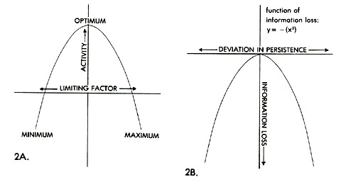
Figure 2. The measurement of environmental stress as interpreted: 1) in Figure 2A, in terms of the zone of tolerance concept of Shelford (1911, 1913); and 2) in Figure 2B, as an indication of information loss. Odum (1967: 109-110) has remarked: "All...kinds of stress...have a common property, that of diverting or draining potential energy flows which would have otherwise led to useful work or storages. Thus we may provide an operational definition of stress as the drain of calories of potential energy flow. One may measure the stress by the change in energy flow of the system, by the disappearance of a previously-existing flow, or even by the acceleration of a repair rate for those systems that can respond to the stress with accelerated energy inflows...a stress...has the effect of moving backward along the limiting factor curve toward its origin... If one turns the axis around, one sees the frequently observed pattern of the dosage response curve for radiation, drugs, pollutants, (and) poisons in operation...Thus a generalized concept of stress, limiting factor kinetics, and dosage response turn out to be the same property of energy reception."

    [[p. 89]] Van't Hoff's rule states that for every ten degrees Centigrade rise in temperature, the general rate of biochemical reaction approximately doubles (Vernberg and Vernberg, 1970). This provides the basis for a post-multiplier that can be attached to the subtotal calculated above to complete the stress index. The multiplier can be derived by choosing an appropriate "mean conditions" temperature as a standard, and converting any location's mean environmental temperature to the multiplier for that location via Van't Hoff's rule. Thus, if we apply as the rational standard from which to measure deviation the mean temperature (energy conditions) at the surface of the earth, 12.5 degrees Centigrade (Sellars, 1974), the multiplier for location ij can be computed from:

M = 2.0 exp ,

where:

"exp." = ((mean annual temp. at location ij)-12.5 degrees C) / 10.0 degrees C.

Net stress at location ij thus becomes s_ij multiplied by M, where s_ij represents the irregularity of resource availability (inherent in the persistence characteristics of moisture supply) at location ij, and M represents a measure of the degree to which the resources available are optimized by promoting spatial interaction.

    It is arguable that the index derived above might be improved upon in a number of respects, but for the present I have decided to apply what I feel is the simplest measure capable of identifying the spatial relationships I will posit should exist. Thus, though the decision to use a single year's moisture budget as the basis for the measure can be questioned, a response to this criticism can be forged by noting that: 1) the yearly cycle of [[p. 90]] climatic variation is probably by far the most significant exogenous factor forcing adaptive response by organisms; 2) additional constraints can always be specified and added ex posteriori into explanatory models; and 3) means exist by which the effect of longer-term exogenous stresses on distribution patterns can be identified independently of a particular rendering of a surrogate for stress (see Chapter VII). (It is also advisable, I believe, to keep the initial means of measuring stress simple so that its imperfections can be more specifically linked to particular parameters, and thus more easily reduced through adjustment (Levins, 1966). For example, Van't Hoff's rule generalizes a relationship that is known to vary considerably (Vernberg and Vernberg, 1970); data-fitting will be necessary to elicit the value most appropriate to the model's needs).

Data Used in the Empirical Studies

    In order to apply some tests to the overall model, a study area was chosen within which a series of pattern analyses was performed to link organismal distributional data to the spatial distribution of stress values. The choice of study area was constrained by several factors. First, the area had to be one for which good distributional and climatological data were available. Second, the area had to be quite large and contain a good variety of ecological conditions, lest the general applicability of the model be called into question regardless of the empirical results. Third, the area had to be reasonably topographically uniform. Although the model should in theory apply under any topographical conditions, the problem here is sampling error. Ecological conditions usually vary altitudinally much more rapidly than they do areally, and for large study areas it is impossible to design a spatial sampling method that accounts for this when [[p. 91]] relevant empirical data are not available (a similar problem is involved in the classification of climates in areas of high relief). The area chosen consists of an expanse of land east of the Rocky Mountains and west of a line approximately following the meridian 80 degrees west. Most of the area is in the United States (see Figure 3); it covers in total approximately 1.5 million square miles. It is an area of relatively regular physiographic character containing a great diversity of climatic conditions; moreover, associated with it is a spatial data base of biota and climate that is reasonably reliable and complete.

    Choice of organismal distributional data was also constrained by prior considerations. First, I wanted to examine the distribution patterns of several different groups to make comparative studies possible. Second, I needed a rather large data base, since the relationships I hoped to uncover were likely to be masked by a large number of external considerations and afflicted with high noise levels. Third, the distributional data had to be relatively precise; that is, substantiated by a considerable record of observation. Fourth, I wanted to treat all the members of the particular groups chosen and to use single references for each in an effort to avoid possible associated biases. The groups eventually selected were the vertebrate classes Mammalia, Reptilia, and Amphibia. Of these, there are, respectively, 205, 165, and 114 species whose ranges extend into the study area. Birds and fishes were not considered because of the possible complicating effects of split range associated with the former, and the non-terrestrial habitats associated with the latter. The sources for the distributional data employed were Hall (1981) for mammals, and Conant (1975) and Stebbins (1966) for reptiles and amphibians.

    A sample grid was applied to obtain the operational geographical units

[[p. 92]]

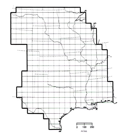
Figure 3. Geographic sampling grid superimposed on the area (outlined in heavy ink) selected for empirical study of distribution patterns of mammals, reptiles, and amphibians.

[[p. 93]] ("OGU"s": Crovello, 1979) used to order the data that were to be related statistically. The values eventually assigned to each cell (for example, the calculation of spatial derivatives: see Appendix 1) can be defended on the basis of a study by Snyder (1983) and information obtained from a review by Haralick (1979) suggesting that the (structural) approaches employed generally yield as good or better results than other methods used to examine texture. The study area divided into 306 areal units (cells), each a square approximately 5000 square miles in area (with the exception of a few of those bordering the Gulf of Mexico and Great Lakes, which were somewhat smaller). The 5000 square mile size was arrived at from considerations dealt with shortly in the section on sources of measurement error.

    Two fundamental kinds of data were collected. The stress field for the area was constructed by: 1) calculating the stress index values from climatological data published for 566 locations distributed fairly evenly throughout the study zone; 2) transforming the longitudes and latitudes of these into coordinates projected onto a two standard parallel Lambert map projection; 3) transforming the latter into SYMAP (Dougenik and Sheehan, 1979) coordinates; and 4) using the coordinates and associated values to produce an isoline map via the SYMAP routine "F-MAP." Various measurements were then retrieved directly from the map on a cell-by-cell basis after the sampling grid was applied. The species distribution maps present in the original sources were recoded into bits on a cell-by-cell basis as well. This was accomplished by projecting the sampling grid over the maps and simply noting presence/absence of each given form in each cell of the grid. Any cell in which both presence and a range limit occurred was noted and coded as such. Recoding of generic and familial level data (created as simple aggregations of species level data) was carried out in analogous [[p. 94]] fashion. All told, about 250,000 primary bits of presence/absence data were recorded.

    Interpretation of the empirical studies to be described in Chapter VI was complicated by the various sources of noise implicit in the type of raw data collected here and their secondary transformations. A number of possible imperfections of measurement exist. The soil moisture data employed to generate the stress index values compiled by C.W. Thornthwaite Associates (1964) have unfortunately been based on meteorological station records of varying length and historical period. Although the climate changes over the approximately 100 year period involved (1860-1960) have been relatively slight, they have not been trivial, and it has been necessary to omit from my derivations those stations in the study area whose soil moisture budgets were based on data not representative of the 100 year period as a whole. The range distribution data suffer from a similar problem, since the range maps are summaries of collections of specimens made throughout a period of about 100 years, and one must expect that the range of many forms has changed some over this interval. This problem must simply be accepted, though I have attempted to minimize it by employing a large number of cases in my hypothesis tests.

    A second problem is related to the first. Measurement accuracy is an ever-present annoyance regardless of the type of analysis to be performed; it can only be accepted here, for example, that some of the meteorological stations have kept more accurate records than others, for whatever reasons. Range data are even more subject to error, since it is to some considerable degree a subjective decision how many recorded presences of an organismal type throughout a given area are needed to designate official "occupation" of the entire area by the form. Nonetheless, in sum the two sets of records [[p. 95]] (climatological and distributional) seem about equally reliable, and with no major identifiable systematic bias. The fact that the range patterns have been "smoothed" to a certain degree by the grid cell sampling process is also a potential problem, though one of the original constraints on the cell size chosen was that it should not be so large as to conceal local correlations nor so small as to overemphasize them. Unfortunately, there is no literature that I have been able to find that is helpful in the present context in making a priori decisions regarding this trade-off. The texture literature (see review by Haralick, 1979) focuses on the identification of pattern characters rather than quantification of same; the spatial filtering literature provides some guidelines regarding measurement of the trade-off function (see, for example, Gaile and Burt, 1980; Mardia, 1972), but cannot provide an initial decision-making framework regarding choice of cell size in the absence of a prior theoretical position. We are thus left in the end with a subjective decision to make regarding choice of "best" coarseness of the grid. This weakness can eventually be overcome by recourse to "best fit" empirical approaches, but time and resources prohibited such here. In any case, the cell size chosen provides a large enough field for purposes of statistical analysis, and the filtering characteristics (e.g., response function) associated with its application could at least be described if necessary to provide an idea of the kinds of biases it imposes.

    The credibility of the Thornthwaite system as an indicator of surface moisture conditions has been treated by Curry (1965). Curry concludes that despite criticism to the contrary (for example, Chang, 1959; Sibbons, 1962), the potential evapotranspiration term remains an excellent estimator (as indicated by spot comparisons with empirical measurements of evaporation) as long as the period for which it has been calculated is sufficiently long and [[p. 96]] representative. This still does not make it the perfect surrogate, but I am unaware of any single measure that better suits the present model, whose application to empirical tests necessitates absolute measures of the climatological state-space rather than relative ones (such as the Palmer Drought Index).

    Measurement errors associated with data transformations may also be expected to have generated noise in the empirical results about to be presented. The Lambert base map used here is not an equal area map; therefore, the absolute size of each cell in real world terms varies within a range of about five percent. (It would have been extremely laborious to convert the distributional range data, which were also plotted on Lambert projections, to equal area representations.) There is in addition always the chance that there have been mis-recordings, and mis-recodings, of data.

    A final source of error devolves from a random element inherent in the structure of the model itself. I have assumed for purposes of simplicity (and in concert with the individualistic hypothesis) that upon arrival at a given location, all populations will find themselves equally unsuited for immediate assimilation into the particular community conditions there. In reality, however, for any given locational situation there is likely to be some range of such relative degrees of unadaptedness. By chance, some forms may exhibit degrees of preadaptation that will enable them to assimilate into community structure easier than one would expect simply by considering their overall adaptive flexibility (here, the magnitude of their identifying K parameter). Others will likely be affected in the opposite fashion. Moreover, the degree of preadaptation (and "negative" preadaptation) in a given population is likely to vary spatially; i.e., with respect to location-specific community conditions. I am assuming, however, that this [[p. 97]] effect will be a random one in space: it seems highly improbable that some very large number of forms will be equally preadapted to large numbers of particular locational conditions independent of the stress factor. Given this assumption, empirical analysis of the significance of range boundary location and diversity characteristics can proceed under the claim that the model specifying predicted relationships is imperfect, but not highly biased.

[[p. 98]] VI. SOME EMPIRICAL TESTS OF THE MODEL

Introduction

    [[p. 98]] Before we proceed to description of the empirical tests of the model presented here, a short summary of the underlying relationships posed should be given. Figure 4 aids us in this endeavor.

    This diagram resembles Figure 1 in its depiction of abiotic and biotic sectors of the earth's surface system, but is more explicit in its inclusion of an extra feedback loop expressing the posited role of spatial interaction in the system's evolution. In earlier discussion, it was advanced that movement through space accompanying the day-to-day maintenance of an organism's individual energy budget increases net system information levels by cumulatively feeding back to reduce energy output demands on the biotic sector in the long-term sense. In Figure 4A, the homeostatic function of adaptations is portrayed. Total energy input and output to/from each sector balances per time period considered. Note the addition of an inferred (and from a strictly physiological point of view, irrelevant) loop depicting flow of energy and resources available to the biotic sector, but not used by it. In Figure 4B, the homeorhetic function of adaptations is portrayed. If we wish, we can equate biological activity with spatial interaction, forcing a cross-sectional view in which, for a given period of time, rates and form of spatial interaction within the biotic sector are understood as being a direct function of the spatial-temporal characteristics of availability of energy and resources. Alternately, we may adopt an evolutionary point of view in which spatial interaction is viewed as producing the by-product of non-random mass redistribution. The potential energy inherent in this

[[p. 99]]

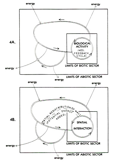
Figure 4. Expanded state-space (4A) and process views (4B) of earth surface system organization, per Figure 1. See text for explanation. Note that double lines indicate path of both mass and energy; single lines, energy alone.

[[p. 100]] redistribution is in effect "used" to reduce that portion of the flow of energy and resources available to the biotic sector that ends up not being used by it (a process of resource cycle "tightening" amounting to stress reduction).

    I see no way of directly testing the idea that the potential energy feedback loop depicted in Figure 4 exists. Direct biological tests (i.e., involving analysis of the biology of organisms or populations) are out of the question, because the adaptations that must at one level or another be the focus of biological inquiry individually contain almost no information relevant to the sum process envisioned (recall the passage from Maruyama (1963) regarding the difficulty inherent in attempts to build normative models from historical descriptions of process). Nonetheless, indirect tests of the hypothesis are possible. Given the assumption that spatial order devolves as a function of ordered processes, we can attempt to demonstrate that the stress field is responsible for ordering the biotic sector into predictable spatial patterns. Success in this attempt will at least support the position that potential energy is being produced, and accepting this will pave the way for any number of more biologically-oriented studies involving the spatial arrangement of attributes. The latter cannot be investigated first because we have already allowed ourselves the assumption that change in distributional range mirrors evolutionary change in general, and to abandon this position before demonstrating that distributional patterns can in fact be interpreted as having resulted from the process posited is to regress toward the adaptation (process) yields adaptation (structure) circularity.

    As earlier discussed, the innovation diffusion interpretation of range change is amenable to either probabilistic or deterministic forms of [[p. 101]] modelling. Thus, an innovation (population) diffusing across an MIF can be equally easily viewed as responding to varying probabilities of extension in different directions or different gradients in different directions. In the model presented here, downgradient diffusion is weighted as much more probable than upgradient diffusion (a fundamental supposition, since it is this preferred extension in direction of lower stress that yields net gains over time in the amount of negentropy imported to the biotic sector). Supposing a relatively unchanging stress field controlling the diffusion of a reasonably large number of innovations (populations) over a non-trivial amount of time, four basic predictions about the nature of the patterns resulting can be made:

1) Low-stress areas should contain a greater number of boundaries per number of forms present. This pattern in theory results from the tendency for ranges to expand away/regress from high-stress areas.

2) Stable high-stress areas should tend to be populated by a larger proportion of forms with small distributional ranges than low-stress areas, a consequence of the ability of high-parameter K forms to diffuse further distances downgradient per unit time than low-K forms.

3) It should be possible to identify similar patterns of response by groups of populations even if they are in general characterized by greatly differing K parameter values. (This prediction does not conflict with the last prediction because in that case absolute differences are predicted within groups, whereas here, relative similarities are predicted across groups.) This is the straightforward consequence of the supposition that topography of the stress field influences direction of range change, but has no direct control over mean rates of change.

[[p. 102]] 4) It should be possible to link the spatial interaction structure of the study area, expressed in terms of faunal similarities values between cells of the sample grid, to the topography of the stress field. Because range change across steep gradients in the field is supposed to be more difficult/time-consuming, we should expect to find that where gradients are low between adjoining cells, faunal similarities should be high (a "corridor" effect: Simpson, 1940).

    These four hypotheses and a number of corollaries and other more specific predictions were tested using statistical procedures, especially multiple linear regression. All the analyses made use of routines from the SPSS library (Nie et al., 1977).

    The casting of these and other hypotheses to be discussed has been strongly influenced by whether the underlying deductions involved thinking within a state-space or process-oriented mode. In the case of state-space formulations, the characteristics of observed patterns of distribution are viewed as being time-independent; that is, as involving measureable correlations over space that should exist regardless of organism type, historical reference frame, or spatial reference frame. The directly process-related deductions are perhaps less diagnostic but invite useful comparative studies, particularly among the general groups of organisms considered here. Thus, in these tests attention is drawn more to the relative states of present distribution among groups with the idea in mind that variations in underlying diagnostic parameters, operating through time, will produce certain systematic differences in distribution patterns.

    Three main sets of variables contributed to the tests. The first consisted of the distributional data, by organism type and taxonomic level, [[p. 103]] and secondary transformations thereof. These ordinarily represented the dependent variables in the statistical analyses. The second consisted of a set of measurements compiled directly from the stress field on a cell-by-cell basis, including the mean, standard deviation, and range of stress values for each cell, and a number of other such measures (see Appendix 1 for a list and description of all the variables employed in the study, and Appendices 2A, 2B, 2C, 2D, and 2E for mappings of the five stress field measures most used). The third consisted of independent "site factors" likely to affect distributional characteristics for reasons largely independent of the present model. Some of these were invoked to account for barrier effects; for example, presence of large rivers, nearness to the ocean, etc. Latitude of cell was included as a site factor as a surrogate for total energy available to the system at the given location. Altitude and range of altitude were included to account for range of environmental conditions within a given cell; this neutralizes the complicating influence that altitudinal zonation over short horizontal distances would otherwise have on the meaning of diversity figures. (See Appendices 2F and 2G for representative mappings of site factor variables.)

    Ordinarily, analysis proceeded by posing some distributional state as the dependent variable to be explained by the combination of stress field-related variables and site factor variables. Usually, the effects of site factors were removed first in the regressions as a gesture to conservative interpretation. In almost all cases, each regression model was run in several different forms, using only some of the 306 cases and/or using different combinations of the independent variables and/or principal components in an effort to reduce multicolinearity and test robustness of results. Space permits the reporting of only the most conservative of these [[p. 104]] tests in Tables 1 through 9. Where the results attained from the use of different suites of variables are markedly different, this is mentioned and discussed in the main portion of the text. Because many of the analyses proposed bore results relevant to more than one of the main and/or secondary hypotheses being examined, it is unfortunately not possible to report the overall results in terms of each hypothesis. At the end of this chapter, however, a summary is presented. Each of the individual studies carried out will now be discussed in detail.

Analysis One

    One of the most important ways in which the relevance of the overall model can be tested is through the study of the pattern of boundaries. Originally, I had planned to examine the boundaries-stress field relationship in terms of correlations of linear patterns; this approach, however, proved to be both difficult to operationalize and rather inflexible. Instead, number of boundaries per cell (for given taxa) were recorded (variables BBOUNi), and these values were predicted from a set of independent variables via multiple regression (see Appendix 2H for a representative mapping of BBOUNi).

    The most straightforward prediction about boundaries that can be deduced from the general model is that there should be relatively more of them--regardless of the group studied and independent of historical biological conditions--in low stress areas, once the absolute diversity of forms (BDIVi) present and site factors are accounted for. This hypothesis is based on the prediction that direction of range change should tend to be downgradient across the stress field. Therefore, the centers of distributional range should tend to be correlated with high stress areas, [[p. 105]] with their boundaries falling in the low stress areas. (It should be added that this assumes a relatively stable climate regime over the area studied for at least a few thousand years and a suite of populations under consideration that do not have many very small distributional ranges and just a few large ones; both conditions are fulfilled here--see discussion in Chapter VII).

    Table 1 shows that this expectation is overwhelmingly confirmed. Variable ZMSTRS, mean stress, has the expected negative sign in the regression equation of all but two (MAMFAM and TURFAM) of the twenty-seven groupings. Of the nine species level regressions (which are of most concern here), ZMSTRS is significant at alpha = .000 in six, at alpha = .010 in one, at alpha = .075 in one, and at alpha = .150 in the last.

    A second pair of hypotheses raised concerning variables that should be relevant to the prediction of number of boundaries per cell could not be strongly confirmed in this particular analysis. According to the model, downgradient dispersal should be associated with irreversible changes in the gene pool of the population in question. Moreover, a steeper gradient should produce slower range change (as more change is required per distance extended). In areas of high stress gradient, therefore, we should tend to find more boundaries. Further, areas of high change in gradient should tend to attract more boundaries, since these will be areas in which range extension will tend to slow or stop, regardless of population and the value of its K parameter.

    Unfortunately, direct prediction of these relationships through regression methods generates weak tests in the present context because of the probable interference of cumulative historical effects on the pattern of boundary location. As it turns out, ZGRAD (stress gradient) displays no

[[p. 106]]

[[p. 107]] pattern of the predicted significance in the regression equations. ZCGRAD (change in stress gradient), on the other hand, emerges with a positive sign in eight of nine of the species grouping regressions. (Interestingly, seven of nine of the families groupings regressions produced a ZCGRAD parameter of negative sign--this fact will be explored later.)

    It only occurred to me later that the conditions described in the last two paragraphs might be examined from an entirely different angle. This analysis, and the interesting results it produced, are reported in Chapter VII.

    The first results of analysis one were confirmed to some extent in correlation analyses in which boundaries per diversity ratios were correlated directly with ZMSTRS. 22 of 27 correlations were negative (as would be expected), including seven of the nine species groupings.

Analysis Two

    To obtain a better view of distributional characteristics at the local level and their relation to characteristics of the stress field, an analysis was carried out linking: 1) the difference in mean stress between cells, to: 2) associated faunal similarities between cells. The main instrument of analysis was simple correlation.

    The historical interaction problem between mean stress and gradient of stress alluded to in the last section could be largely avoided by performing analyses specific to each cell, and thus focusing on very local time-space relationships. The fundamental hypothesis was that faunal similarity between a given cell and one of its surrounding cells should be less where the difference between that same cell's mean stress and the second cell's mean stress is greater. For each cell and its set of surrounding cells, [[p. 108]] therefore, a set of such comparisons should yield a negative correlation. The reason, again, has to do with the greater likelihood that a steep stress gradient should tend to reduce rate of integration of populations into community structure (and thus tend to separate populations from one another).

    The first step in carrying out the test for each set of nine cells--that is, a given cell and its surrounding eight cells (excepting boundary cells, for which less than nine cells were involved)--was to obtain the differences in mean stress for the eight pairings of the center cell with its neighbors. For each three by three matrix of adjoining cells, the differences were calculated as:

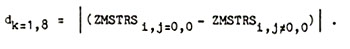
    The complementary faunal association values between the center cell and its eight neighbors were calculated using the simple method described in Smith (1983a). Each set of eight similarities was derived from:

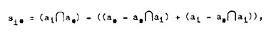
where s_i* is each similarity value between the center cell (i) and one of the other cells (*). Note that the faunal similarity of a cell with an identical cell is the absolute diversity of that cell (BDIVi). Next, the difference between each faunal similarity and the absolute diversity of the center cell was taken, yielding 306 sets of eight values that could be directly correlated with the 306 sets of mean stress differences recorded earlier.

    A summary of the (summary of) results appears in Table 2. Fourteen sets of 306 correlations (ECORRi) were calculated. In thirteen of the

[[p. 109]]

TABLE 2

SUMMARY OF CORRELATION ANALYSES LINKING LOCAL CONDITIONS OF STRESS FIELD TOPOGRAPHY TO
LOCAL FAUNAL ASSOCIATION PATTERNS (ANALYSIS TWO)

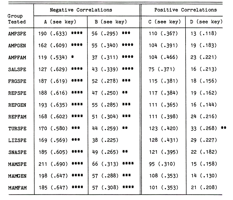
Key:  A = total number of negative correlations recorded, with proportion of all correlations represented; B = total number of significant negative correlations recorded (alpha = .200), with proportion of negative correlations represented; C = total number of positive correlations recorded, with proportion of all correlations represented; D = total number of significant positive correlations recorded (alpha = .200), with proportion of positive correlations represented; significance levels: "****" = significant at alpha = .000, "***" = significant at alpha = .010, "**" = significant at alpha = .075, "*" = significant at alpha = .150; variables and regression names explained in Appendix 1.

[[p. 110]] fourteen studies, there were significantly more negative correlations than positive correlations appearing at a significance level of .010. Further, the number of correlations that were negative and significant at alpha .200 were themselves significantly higher than would be expected (at alpha = .075) in all but one of the fourteen studies.

    These findings are good evidence in favor of the notion that the topography of the stress field as here defined influences rate of faunal interaction between adjoining areas. To strengthen them, however, extensions of the analysis were also performed.

Analysis Three

    The first extension of analysis two involved working with the standard deviations (ESDEVi) of the eight faunal similarities values associated with given cells and their surrounding neighbors (see Appendix 2I for a representative mapping of ESDEVi). Generally speaking, one might expect three things to be associated with larger standard deviations: 1) low mean stress (ZMSTRS); 2) high rate of change in stress gradient (ZCGRAD); and 3) high range of stress (ZRSTRS). Lower stress areas will tend to have higher values of ESDEVi because they will have relatively more boundaries to begin with (per earlier discussion). The other two relationships are likely to be weaker ones associated with the idea that cells in areas of high local topographical variation in the stress field will tend to have higher faunal similarities in some directions than others due to the directional channelling effect of gradient.

    In the fourteen analyses run (see Table 3), all predictions were to one degree or another fulfilled. Mean stress was an important predictor (significant at alpha =.075) in all but one model. Moreover, the sign

[[p. 111]]

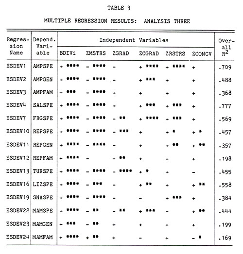
Key:  "+" and "-": sign of Beta values in multiple regression equation; "***", "**", and "*": significance at alpha equals .000, .010, .075, and .150, respectively; variables and regression names explained in Appendix 1.

[[p. 112]] predicted was correct in all but one (unfortunately, the one positive sign recorded was also significant at alpha = .075; however, this was at the family level of aggregation). The sign of the other two variables was predicted correctly in twelve out of fourteen analyses, the variables being significant at alpha = .150 in 11 of the 28 studies.

    These findings constitute weak, but not insignificant, reinforcement for the findings discussed in the description of analysis two.

Analysis Four

    In another effort to validate the results of analysis two, the sets of values EDIFi were used as dependent variables in seventeen regression analyses in which the predictor variables were the combined sets of site factors and stress field measures (see Appendix 2J for a representative mapping of EDIFi). A high difference between given cells' diversities and the means of their eight surrounding cells' faunal association values with the center cell should in theory be associated with: 1) low mean stress; 2) high range of stress; 3) high convexity of local stress surface topography, and 4) high change of gradient in stress. The high association of boundaries with low stress areas again explains the first relationship. The other three positive correlations in theory result from each associated variable's role as an inhibitor to rate of range change, and thus to reduction in rate of interaction.

    The results obtained from the multiple regressions are given in Table 4. The findings are remarkably consistent with expectations, especially at the species level. In fact, among the nine species regressions, only one sign is predicted incorrectly, for variable ZCONCV in the TURSPE model. These findings also strongly confirm the idea inherent in the model that the

[[p. 113]]

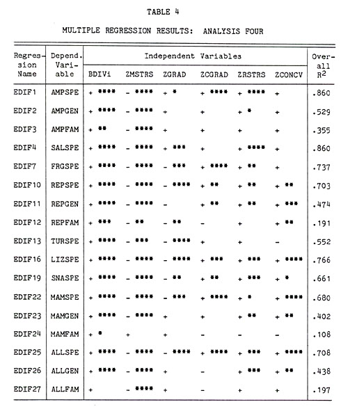
Key:  "+" and "-": sign of Beta values in multiple regression equation; "***", "**", and "*": significance at alpha equals .000, .010, .075', and .150, respectively; variables and regression names explained in Appendix 1.

[[p. 114]] distribution of different groups of organisms can be viewed as a response to basically one set of influencing environmental factors (hypothesis three). A further confirmation of hypothesis three comes from the sets of correlations (ECORRi) involved in analysis two. If one takes the eight sets of 306 species level correlations and correlates them with one another, all of the twenty-five non-redundant correlations produced are found to be positive (with twenty of these significant at alpha = .010). Further, when all non-redundant correlations among EDIFi/BDIVi are determined, 21 of the resulting 23 correlations are positive, with 17 being significant at alpha = .001. Another related bit of evidence is the fact that the variable Z4, which measures mean difference between a given cell's mean stress and the mean of the eight surrounding cells' mean stresses, is negatively correlated. (though not highly) with all but one (FRGSPE) of the ECORRi sets used in analysis two. This suggests: 1) that such mean differences are linked, as would be expected, to the degree of faunal interaction between locations, and 2) that such response is not peculiar to given groups.

    The results obtained in the regression analyses were confirmed further by correlating ZMSTRS with EDIFi/BDIVi. All correlations were negative, as would be predicted, with fifteen of seventeen being significant at alpha .020.

Analysis Five

    A further extension of analysis two involved the prediction of variable sets constructed from variable sets ESDEVi, BDIVi, and EDIFi. The construction predicted was: ESDEVi/BDIVi-EDIFi = "ECVARi"; the elements of ECVARi are the coefficients of variation derived from the means and standard deviations associated with the faunal similarities of the eight surrounding [[p. 115]] cells with a center one. These values were predicted from the sets of site factors and stress field variables.

    One would expect the Betas in the regressions for ZMSTRS and ZCGRAD to be negative and positive, respectively. Areas of low stress are here predicted to be mixing areas where ranges of organisms intersect (in the study area, largely from two directions), a phenomenon that would lead to direction-dependent faunal similarities values and thus high standard deviations. High ZCGRAD values areas should be areas of high directioning of range change at slow rates, again generating direction-dependent faunal similarities and high standard deviations.

    The results (summarized in Table 5) are favorable, if not strongly so (much information is lost in the calculation of coefficients of variation). The Betas for ZMSTRS are of negative sign in eleven of fourteen regressions (including seven of eight of the species groupings), and six of these are significant at alpha = .020 (including three of the species groupings). The Betas for ZCGRAD are of positive sign in nine of fourteen regressions (including six of the species groupings). The results for the ZCGRAD components are strengthened a little by the fact that only nine of fourteen of the simple correlations between ZCGRAD and ECVARi are negative (some partial correlation thus being exposed by the removal of intervening variables).

Analysis Six

    Setting up analysis two and the checks following it required much data file manipulation and was very time-consuming. For this reason, only the simplest tests were applied. Moreover, several short-cuts were taken (for example, assuming that all eight cells surrounding a center cell located

[[p. 116]]

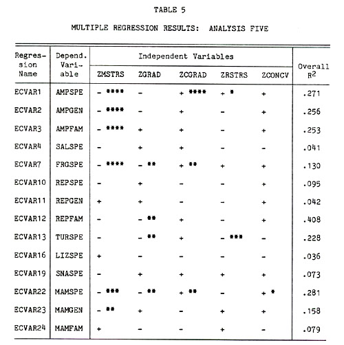
Key:  "+" and "-": sign of Beta values in multiple regression equation; and significance at alpha equals .000, .010, .075, and .150, respectively; variables and regression names explained in Appendix 1.

[[p. 117]] within a row and column matrix were spatially equivalent in their relationship to that cell). The results obtained are therefore considered to be conservative assessments of the relationships studied. In the last extension of analysis two, another short-cut was employed. Ideally, an entire set of studies parallelling analyses two through five might have been applied to cell-by-cell relationships between surrounding cells' faunal similarities and stress gradient characteristics. Instead, only one such study was carried out, for ALLSPE. The same procedure set out in the description of analysis two was employed, the only difference being that faunal similarities were this time correlated with the differences between the center cell's stress gradient (ZGRAD) and those of surrounding cells to produce 306 values of "EECORR." This operation produces a view of the local effect of change in stress gradient on local diversity characteristics.

    We should expect to find in the set of 306 simple correlations resulting a negative relationship between BDIVi=1,306; j=1,8 - EDIFi=1,306; j=1,8 and the differences between given cells' ZGRAD values and those of its surrounding cells. In the actual results, 201 of 306 correlations are negative, with 73 (36.3%) of these significant at alpha = .20. Of the 105 positive correlations, 18 (17.1%) were significant. The difference between these is itself significant at alpha = 0.

    The follow-up multiple regression analysis in which the 306 correlation values were predicted from site factor and stress field variables produced predictable results. Although the overall model was as poor (R²= .067) as those produced in the ECORRi follow-ups, its F statistic was significant at alpha = .037. More importantly, ZGRAD was a significant variable in the regression equation (at .005), and had the expected sign (negative). These results strongly confirm the reasoning that the more negative correlations [[p. 118]] produced in the main part of this analysis should be associated with higher stress field gradients.

Analysis Seven

    A rather different kind of deduction regarding the state-space of distributional patterns can be made concerning entire distributional ranges. If: 1) the general tendency is for populations to extend range in a downgradient direction across the stress field, and 2) populations display varying rates of accomplishment of this act (i.e., have varying R parameters), it follows that: 1) areas of high stress should be populated by forms whose distributional ranges are small in area on the average as compared to those of forms populating low stress areas, and 2) the standard deviations associated with the range areas of all forms present at a given location of high stress should be higher than that for assemblages of forms associated with a low stress area. This will again tend to be true regardless of setting or historical situation, since the topography of the stress field will act as a "temporal filter" denying low-K populations access to low stress areas regardless of how long the diffusion process has been occurring. Refinements of this idea are presented in Chapter VII.

    To test this prediction, a regression format was again employed. The independent variables were the same stress field and site factor measures, but new dependent variables had to be constructed to depict the means and standard deviations of range size of all forms extant in each cell. In the interest of time, a categorical approach was employed. Seven categories of range size were first arbitrarily established: 0-50,000 square miles, 50,000-100,000 square miles, 100,000-200,000 square miles, 200,000-400,000 square miles, 400,000-800,000 square miles, 800,000-1,600,000 square miles, [[p. 119]] and greater than 1,600,000 square miles. The distributional areas of each of the 484 species populations treated in the study were then classed according to this scheme. Finally, for cell-specific faunas means and standard deviations of range areas were calculated. Variable sets KMCSMPi and KSDCSMPi were thus derived for the eight species groupings studied (representative mappings of these statistics are displayed in Appendices 2K and 2L.

    The results, displayed in Table 6, again tend to confirm the expectations, especially for the set of KSDCSMPi regressions. Regarding the latter, all species groupings exhibit positive Beta signs for mean stress in the regression equations, and this variable is significant at alpha = .000 in all eight models except that for lizard species, where it is significant at alpha = .075. The KMCSMPi regressions were almost as successful, with seven of the eight models containing a negative mean stress parameter significant at alpha = .010 (with LIZSPE significant at .010, but positive in sign).

    These sets of tests were also run in three other ways, inserting "latitude" (XLAT) and "absolute diversity" (BDIVi) individually, and then in tandem, as additional independent variables. This has some effect on the reliability of sign of mean stress (ZMSTRS) in the resulting set of KMCSMP regression equations, probably because both tend to be fairly highly correlated with both mean stress and KMCSMPi.

    The most surprising result from this study was the remarkable uniformity of sign and significance of the other four explanatory stress field variables considered. I see no reason for these being statistical artefacts, since none is very highly correlated (see Appendix 3). Moreover, they respond rather differently than does ZMSTRS to the insertion of the

[[p. 120]]

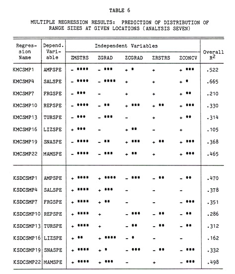
Key:  "+" and "-": sign of Beta values in multiple regression equation; "***", "**", and "*": significance at alpha equals .000, .010, .075, and .150, respectively; variables and regression names explained in Appendix 1.

[[p. 121]] latitude and diversity variables into the equation. It appears that these findings might, however, be interpreted through the model presented here. The positive relation between "mean cosmopolitanism" (KMCSMPi) and ZCONCV, ZRSTRS, and ZCGRAD might be attributed to the fact that all else accounted for, low-K populations, despite their affinity with high change-in-variation-in-stress areas where they do exist, tend to be unable to diffuse to other such areas and are absent from them. In short, some high-stress areas may for historical reasons be more stably so, and "collect" low-K populations, whereas others, of greater recency or intermittency, are unlikely to contain many of these. These themes will be expanded in Chapter VII and to some extent in the description of analysis eight in this chapter.

    The kind of analysis applied in this substudy was also carried to the familial level for mammals. A somewhat different method was employed, however. First, a systematic sample of 40 cells was taken and the mean stress and familial diversities noted for each case. For the measure of net mean cosmopolitanism exhibited by the mammal fauna of each cell, information derived from Smith (1983a) was employed. Each mammal family in the present study area is found in a certain number of the set of world subregions in the mammal faunal regions classification presented in that paper. A distribution of those numbers was compiled for the familial elements present in each of the 40 cells of the sample, and statistics (mean and standard deviation) calculated from these data.

    The forty mean stress values correlated negatively with familial diversity and the mean and standard deviation of the distribution at -.478, -.523, and -.536, respectively (all significant at alpha = .000). Thus, more cosmopolitan and higher diversity faunas tended to associate with low [[p. 122]] stress areas, a finding consistent with the species level results.

Analysis Eight

    This analysis, concerning the rates of occurrence of limited-range populations in space, was performed in an effort to test whether the model presented here could predict under what spatial circumstances such populations tended to collect. Disjunct and relict populations with ranges of less than 50000 square miles were first tallied on a by-cell basis. Nine such tallies were completed (LIMRi). These values were then predicted via regression from the sets of stress field and site factor variables.

    These analyses were frustrated by three problems: 1) the decision not to complicate the analysis by assessing a priori the kind of limited range population being dealt with in each instance (i.e., disjunct population or relict); 2) the historical bias problem discussed in the descriptions of analyses one and seven; and 3) the empirical difficulty of having too many cells with zero values. In general, it was expected that high rates of occurrence of limited range populations should tend to be associated with high mean stress (ZMSTRS) and high variation in gradient of stress (ZCONCV, ZRSTRS, ZCGRAD, and ZGRAD), but these expectations were neither contradicted nor confirmed (see Table 7). Simple correlation analyses of these factors with LIMRi/BDIVi proved only a little more successful. ZGRAD was positive in six of nine cases and significant at .010 in three of these; ZRSTRS was positive in seven of nine cases; ZMSTRS was positive in seven of nine cases and significant at .010 in five of these, and ZCGRAD was positive in seven of nine cases. Interestingly, however, the pattern of limited range populations is correlated among groupings, since 22 of the 23 non-redundant comparisons across species groupings are positive in sign. This is another

[[p. 123]]

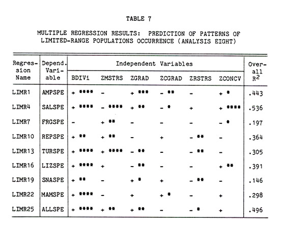
Key:  "+" and "-": sign of Beta values in multiple regression equation; "***", "**", and " ": significance at alpha equals .000, .010, .075, and .150, respectively; variables and regression names explained in Appendix 1.

[[p. 124]] indication of the generally similar response of different groups to the conditions of the stress field topography.

    The generally mediocre results obtained in this analysis suggested that a more involved model was needed. Relevant ideas are presented in Chapter VII, along with the results of a reconstituted empirical analysis.

Analysis Nine

    In this analysis, the areal distribution of boundaries described in terms of genus/species and family/species ratios (= "RATIOi") were predicted from site factor and stress field variable sets. A number of predictions about the spatial distribution of these ratios could be made on the basis of the present model, but only one was focused on here. This concerns the use of variable ZCGRAD to predict intra-generic and intra-familial distributional relationships.

    Given that ZCGRAD influences rates of diffusion across the stress field (and considerable evidence has already been presented to suggest that it does), one can ask the question whether it might also act as an isolating factor between closely related populations. This would seem to be an obvious implication, since gene flow in high gradient change areas would ostensibly be slowed, and such slowing can be considered an isolation process. We should therefore find genus/species and family/species boundary ratios to be lower in areas of high ZCGRAD values, since species boundaries will tend to be more plentiful in these than generic or familial level boundaries.

    Table 8 indicates that these expectations are fulfilled. All nine genus/species ratio regressions produce negative ZCGRAD parameters; six of nine family/species ratios produce negative ZCGRAD parameters. Two of these

[[p. 125]]

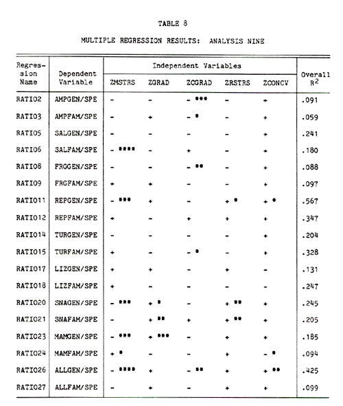
Key:  "+" and "-": sign of Beta values in multiple regression equation; "***", "**", and "*": significance at alpha equals .000, .010, .075, and .150, respectively; variables and regression names explained in Appendix 1.

[[p. 126]] are significant at alpha = .150, and three at alpha = .050. These results are backed up by findings reported in the description of analysis one. In those regressions, it can be seen that there is a strong tendency for the ZCGRAD parameter to change from positive to negative in the regressions predicting rates of boundaries present as one shifts from the species level of aggregation toward the familial level.

    This is an important find, as it strongly suggests that topography of the stress field is a significant factor in the speciation process, and bears on discussions involving consideration of clines, hybrid zones, and population genetics in general (and especially the subject of isolating mechanisms). It is relatively difficult, however, to bring together all the evidence from the pattern analyses that are relevant without considerable further study, and for this reason, discussion will not be further developed here.

Analysis Ten

    In this study, it was hoped that it could be shown that mean orientation of range boundaries within cells correlated with mean direction of slope of the stress field across same. The analysis thus involved deriving 306 such values for each species grouping involved.

    The correlations were phrased as a difference in degrees between the directions of two vectors. The first vector was direction (and magnitude) of stress field slope across given cells; the second was the circular mean (and magnitude) to cell centroid calculated from the numbers of range boundaries facing in north, south, east, and west directions within given cells (see representative mappings of the latter in Appendices 2M, 2N, 20, and 2P). The circular means were calculated from:

[[p. 127]]

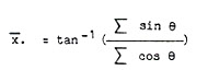
In addition to the circular mean, the circular variance ("CCIRVARi") was calculated for each cell from:

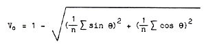
(These equations were obtained from Mardia, 1972, and Gaile and Burt, 1980.) A third set of values, the variances ("CVARi") associated with the range in numbers of boundaries facing in north, south, east, and west directions in each cell was also retrieved.

    Once the two sets of sets of vectors had been derived, their angular differences ("CDIFDIR") were found. These potentially ranged from zero to ninety degrees; small values indicate close agreement between boundary direction trend and stress field trend.

    The immediate results were not very impressive. The means of the eight distributions of differences were all fairly close to 45 degrees, the null hypothesis (with six of eight less than 45 degrees). I blame these indifferent results on several factors, including filtering problems and the possible unsuitability of the mean direction measure, a range boundary direction bias in favor of north and south boundaries, the coarseness of the grid sampling method, the influence of historical considerations, and the a priori probabilistic nature of local range boundary adherence to the stress field topography. hat the measures being compared were very imperfect to begin with is evidenced by the fact that the two measures of stress field gradient directional trend used in the analyses (which were therefore [[p. 128]] actually conducted twice) produced values which for the eight groupings correlated with one another at an average of only about r = .50.

    Nonetheless, some encouragement was squeezed out of the analysis. First, when the elements of CDIFDIRi were grouped into classes of range of angular difference and subjected to a Goodness-of-Fit test based on the null hypothesis of random placement, all eight groupings failed the test at alpha = .150, suggesting that despite the failure of the main test, non-random associations still existed. More importantly, the secondary prediction of CDIFDIRi elements produced some interpretable results. Given the notion that the strength of the values of the elements of CDIFDIRi should secondarily be relatable to the nature of local conditions of the stress field topography, we should expect some predictive power exhibited by the latter, especially variables ZMSTRS and ZCGRAD. These variables have already been shown to influence directionality of interaction among neighboring cells in a different context (the descriptions of analyses two through five). Simple correlations between CDIFDIRi and these confirm this expectation, with seven of eight in each set being of the expected sign, though small in magnitude.

    We can also look at relationships among the different organismal groupings. For example, if the values of CDIFDIRi are indicative of a common response by different species groupings, then these values should be positively correlated with one another. 22 of the 23 relevant correlations are in fact positive, with twelve of these correlations significant at alpha = .150.

    It would have been interesting to apply some more sophisticated tests to the above data, and to repeat the tests already described using the direction of slope of change in stress field slope (t) as the vector to be [[p. 129]] compared with mean direction of range boundaries, but a quick time-benefit analysis of the situation suggested that it would be better to wait for an opportunity to apply more elaborate controls to the system.

Analysis Eleven

    The prediction of absolute diversities ("BDIVi": see representative mapping in Appendix 2Q) from site factor and stress field measures is not in itself a terribly useful thing to do, because BDIVi is not a state-space characteristic (i.e., the spatial characteristics of absolute diversity are themselves predicted to change over the life of the system). However, one can argue that a weak test may be constructed around a comparison of diversity characteristics among species groupings. This notion is based on the idea that different general taxa may be characterized by greatly differing K values, and thus will have been able to extend their range to differing degrees across the stress field.

    Our fundamental expectation should be that groups characterized by high K values will have in general extended their range toward low stress areas more than will have groups characterized by low K values. We must first decide how to recognize the difference between a "low-K" and a "high-K" group. No single non-circular mode of reasoning seems to work here, but three pieces of information can be used in conjunction to provide a certain general ranking. These are: 1) present mean area, of range for species within a given grouping; 2) measured physiological tolerances of species within a given grouping; and 3) known habitat types to which species within a given grouping are limited. A further necessity is the knowledge that elements of all groupings have had access to the area of study for equal periods of time (we would not, for example, wish to compare the diversity [[p. 130]] characteristics of a recently introduced group to those of a long-established group for fear of introducing a compound process bias into the examination).

    The groups examined here--mammals, turtles, lizards, snakes, salamanders, and frogs and toads--seem to fall into a fairly clear order with respect to their K parameter. This order, from top to bottom, is mammals, snakes and lizards, turtles and frogs and toads, and salamanders. A detailed documentation of this classification is possible, but for present purposes it is enough to indicate that: 1) at one extreme, mammal species have larger ranges, are physiologically more flexible, and inhabit a wider range of habitats than does any other living group, and 2) at the other, salamander species tend to be small-ranged and quite physiologically-and habitat-restricted.

    We find in Table 9 that the regressions indicate the sign of the ZMSTRS parameter in the regressions to fit our expectations: it is strongly positive for SALSPE and TURSPE, weakly positive for FRGSPE, weakly negative for SNASPE, and strongly negative for LIZSPE and MAMSPE (it should be noted here that it is the rank-order of the signs, rather than their actual values, that is predicted here; the range of values emerging will be a joint function of: 1) the degree of difference among the K parameter values under consideration; and 2) the nature of the stress field topography involved). Moreover, the simple correlations listed also follow the same general rank-order suggested.

    I admit this to be a weak test, but it is nonetheless an important one, for had negative results emerged here, the model would have been hard-pressed to explain why this should have been so.

Summary

[[p. 131]]

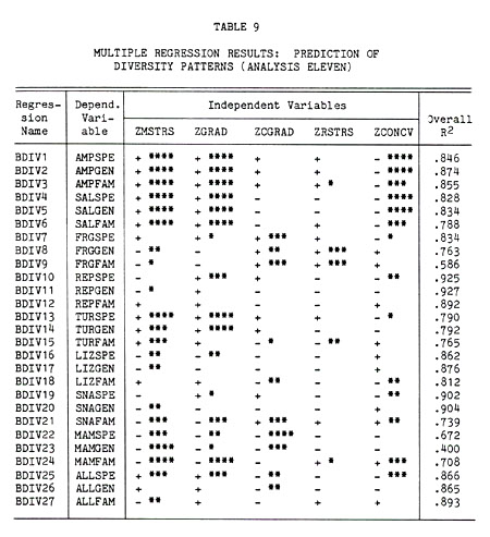
Key: "+" and "-": sign of Beta values in multiple regression equation; "***", "**", and "*": significance at alpha equals .000, .010, .075, and .150, respectively; variables and regression names explained in Appendix 1.

    [[p. 132]] The results described in the preceding eleven descriptions are positive enough, I believe, to suggest that the model developed here has some general validity in the portrayal of the fundamental influences on distribution of organisms. Individually, none of the analyses is strong enough to be diagnostic, but in sum they contribute reasonably strong testimony. Moreover, it should be re-emphasized that, given the various sources of error involved and the simplicity of the tests applied, the results must be considered to be at worst very conservative indications of the relationships involved. A summary of the results of the tests of the main hypotheses follows.

1) Hypothesis one, that distributional ranges should tend to be centered over high-stress areas, is strongly confirmed by the results of analysis one.

2) Hypothesis two, that high-stress areas should be populated, on the average, by forms with smaller total distributional areas, is strongly confirmed by the results of analysis seven.

3) Hypothesis three, that the stress field should influence distributional dynamics in similar fashion regardless of the group studied, is confirmed by the results of virtually all the analyses run. In addition to the regression and correlation studies already described, I attempted a number of other correlations among dependent variables (for example, among the sets of correlations ECORRi discussed in the description of analysis two), and consistently obtained a large majority of positive correlations. Moreover, residual series from each set of regression models were analyzed in like fashion, with similar results being obtained (leading to the conclusion that [[p. 133]] even those aspects of the distribution patterns not explained by the regression models can be explained in a single fashion across groups).

4)Hypothesis four, concerning the micro-interaction structure of the system, was confirmed in part. Analyses two through six were on the whole successful in exposing the patterns expected, but there is still the inconsistency that the variable ZGRAD usually behaved as expected (analyses two, three, and five) but once did not (analysis one). Materials presented in Chapter VII, however, suggest the source of the difficulty.

    In addition, the four more limited hypotheses tested in analyses eight through eleven returned mixed results. Eight and eleven were on the whole successful, suggesting, respectively, that gradient characteristics of the stress field do induce isolation of populations and that total diversity patterns can be linked to group-level K-parameter values. Nine and ten produced few interpretable results, but the chances are good that test model specification and/or variable measurement problems are at fault.

    It is also possible to state pictorially, in idealized fashion, the most important results of the pattern analyses. This is attempted in Figure 5. There, three imaginary genera comprised of three, five, and three species, respectively, are plotted on a likewise imaginary stress field surface in a fashion relaying some of the characteristics apparently displayed by the actual distribution of forms in the study area. As a final review of findings reported in this chapter, several general relationships may again be pointed out (it must be realized, however, that Figure 5 is a rendition of observed associations, and not an attempt to provide a realistic statistical synopsis of findings: to accomplish the latter, overlapping portions of ranges of other genera/species extending beyond the

[[p. 134]]

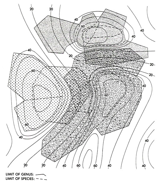
Figure 5. Patterns of distribution of three hypothetical genera (and associated species) consistent with the general findings reported in Chapter Six. See text for discussion. Numbers labelling isolines indicate stress magnitude.

[[p. 135]] map and not portrayed here would have to be included).

    With respect to areal considerations, it will be noted that the high stress areas in Figure 5 tend to have both a greater range of sizes of distributional ranges and a smaller mean size of same than do low stress areas (per analysis seven). Further, distributional ranges tend to be centered over high stress areas more than over low stress areas (per analyses one and seven).

    With respect to boundary associations, it is indicated that boundaries of species populations tend to cluster in areas of high change in gradient of the stress field (per analysis one) and tend to line up more with one another in the same areas (per analyses three, five, six, and ten). Further, generic level boundaries, while also tending to be greater in number in low stress areas, tend to be reduced in number in areas of high change in gradient (per analysis nine).

[[p. 136]] VII. EVOLUTION AND THE RECURSIVE DEVELOPMENT OF DISTRIBUTION PATTERNS

    The results of the empirical tests discussed in Chapter VI on the whole support the contention that normative modelling of the factors underlying organismal distribution patterns is possible. This kind of common basis for approaching problems has not been possible in biogeographic studies before now because of the inability of workers to settle on a means of directly connecting state-space controlling elements to a historical reference frame. Here the concept of the stress field has been introduced to provide a standard for the study of cross-sectional states of distribution; the historical reference frame is specified by the explicit conditions of change within a population (both spatial and genetic/adaptive) produced by its movement (range change) across the field.

    In this work we have so far not dealt much with the complication that the topography of the stress field itself might vary with time. That this must occur is as obvious as the existence of climatic change. The studies described in Chapter VI were performed under the assumption that climatic change of substantial magnitude (at least as compared to the range of conditions now existing) had not occurred in the study area for some thousands of years (enough time for populations' distributions to have responded to the deterministic stress field element). In this instance I believe such a stance is reasonable (see later discussion in this chapter). In many or most other geographical settings, however, we must aware of the possibility that even slight changes in climate within an area, if coupled with an initially relatively unpatterned stress field topography, will render application of some of the pattern analysis approaches discussed so [[p. 137]] far inadvisable (or at the least, their meaning incomplete). Attempts to ignore the fact that state-space-controlling factors can themselves change can lead to fallacious understandings (such as the "age and area" hypothesis of Willis, 1922; Gleason, 1922).

    Nonetheless, this should not prevent us from applying the logic of a particular model to the interpretation of time- and space-linked situational relationships. This has been the method of historical biogeographical analysis all along, and there seems no reason to call for change. The difference between past efforts and the mode of examination to be considered here, however, is that the present logic: 1) involves more explicit initial statements about the controls set by environmental conditions on population distribution and its evolution, and 2) envisions such evolution as being of a single type across all organisms, though varying in its rate. These advantages make it possible to consider a variety of problems from a single, nomothetic, perspective.

    The discussion that follows ranges over a wide range of subjects. In general, however, it is devoted to a consideration of the way interaction of populations and environments might yield patterns of distribution under conditions of changing stress field topography. Many of the remarks may be adjudged as highly speculative; nonetheless, I maintain that they can be subjected to empirical test, and in support of this some samples of such study are also presented.

Vicariance Events, Speciation, and Evolutionary Equilibrium

    It should be remembered that earlier criticism regarding the role of vicariance biogeography in biogeographical studies was not meant to apply to the concept per se. On the contrary, the vicariance perspective appears to [[p. 138]] me a long overdue balancing of the classical view that speciation is a process linked largely to active dispersal events. Both Darwin and Wallace attributed much importance to the role of dispersal (Fichman, 1977, 1981); this view was amplified over the next one hundred years to an extent that proper attention was not given to the possibility that passive speciation events might contribute significantly to the evolutionary process. Wallace, at least, had attributed the process of disjunction to the intervening evolution of barriers to movement coupled with range regression (for example, in Wallace, 1860), but then-current ideas on the general permanence of the great land masses encouraged dispersal-dominated conceptualizations of the diffusion of evolutionary innovation (an influence that Wallace himself later fell victim to). This trend was also fueled by the attention Darwin and Wallace gave to the varying dispersal potentials of animals and plants (Semper, 1881; Ghiselin, 1969). With Croizat's work and the emergence of continental drift as the preferred vehicle for reconstructing paleogeographical settings, however, the stage was set for re-interpretation. Hennig's philosophy of systematics provided the final impetus, since through it derived character traits could be related to allopatric speciation and a specific spatial arrangement of pairs of distributional ranges.

    In this discussion, I should like to concentrate on two issues related to vicariance biogeography. The first concerns the actual occurrence of vicariance events; the second, the relation of vicariance events to dispersal events.

    Croizat's (1958, 1962) observations on the worldwide distributions of a number of forms led him to conclude, as mentioned in Chapter II, that in many cases barriers to dispersal represented the centers of regional [[p. 139]] assemblages rather than the boundaries of same. From this it was a short step (for example, to Croizat et al., 1974) to propose that the evolution of barriers subsequent to an initial placement of populations was responsible for the isolation factor leading to speciation. This contrasted with the classical view that populations tended to disperse into an area, become isolated as a result of pre-existing barriers, and then to diverge.

    The most obvious kind of vicariance-causing event is that in which a previously single land area is severed into two new areas by the evolution of a water barrier such as a lake or arm of the sea. Only slightly less obvious is the effect that rapid mountain-building might have on the isolation of populations. The same can be said for major displacements of large rivers. Most interesting to consider, however, are those situations in which vicariance might be initiated by climatic change. We might, for example, posit the distribution of a particular pair of sister species populations to be the result of a past acidification event that occurred over the central portion of a single parental population, splitting the latter into new, geographically-distinct, subpopulations (see an interpretation of this type by Cracraft, 1982a). The discrimination of such episodes is contingent on parallel reconstructions of the phylogenies of the organisms involved (and ordinarily more than a single pair of co-spatial sister species are sought) and the physical circumstances involved (see Platnick and Nelson (1978) and Rosen (1978) for relevant methodological discussions).

    It is difficult enough in most instances to unambiguously reconstruct both a set of phylogenies and the environmental evolution characteristics relevant to the consideration of particular vicariance episodes. But even success in these operations does not touch upon the matter of what is going [[p. 140]] on at the ecological level as a vicariance event takes place. Vicariance biogeographers, most of whom have little or no interest or background in ecological or population biology studies, have given little attention to this aspect of speciation. Yet it is clearly an important matter for evolutionary studies in general, as speciation is still not a well-understood process, especially at the ecological level (Endler, 1977; Aarssen and Turkington, 1982). The model under study in this work can be helpful here, I believe, in several respects.

     Let us first imagine an area of total environmental stability, and that coextensive with it exists a species population whose range is essentially unchanging; that is, the population has reached a relationship with its environment in which its individual contribution to heat entropy production is being maximized (i.e., R = 0). This situation is depicted in Figure 6A. Next let us suppose, as is shown in Figure 6B, that for reasons unimportant a sudden climatological change occurs over the center of the organism's range, and that this change results in an increase in stress levels there.

    This change in environmental conditions will demand a response at the community, and, ultimately, the population level if state-space equilibrium is to be maintained. I have already assumed that the population of interest had been functioning under R = 0 conditions; that is, that it had reached a state of indefinite reproduction of its own genetic constitution. Regardless, the conditions of heightened stress will dictate change; if the stress-increasing event has been too severe, behavioral and phenotypic shifts may not be enough to deal with the situation, and the population may be extirpated in some areas. Importantly, it is predicted here that it will tend to fail first in those places of greatest change, which in the case of

[[p. 141]]

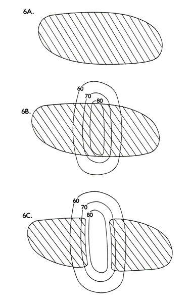
Figure 6.  Disjunction of species population range by intervening climatic change. In 6A, the initial conditions are specified, including a stress field level that is the same across the entire range of the population. In 6B, climatic change has produced a new stress field topography characterized by high stress levels across the center of the range. In 6c, the result of the new stress field topography--a disjunction--is indicated. Numbers labelling isolines indicate stress magnitude.

[[p. 142]] the situation depicted in Figure 6 will be through the center of the range. (We can expect this because these will be the places at which the most significant changes in spatial interaction patterns will be forced; note the related comments on stress definition given by Odum (1967) in Figure 2.) As a result, the population will be split into two new populations (Figure 6C).

    We do not yet, however, have a vicariance event. The result, in fact, is simply a pair of disjunct populations of the same species. Moreover, they will stay that way, because I have already suggested that their degree of specialization has precluded further significant adaptive adjustments. This example, however, must be considered to represent an unlikely set of real world conditions. Let us next consider some more likely ones.

    Climates are never so constant over long time periods as to produce levels of stress that do not change. Biotic potential is similarly variable through time. Like geomorphological systems (which they are in a sense, if one understands the systems approach espoused here), biological populations seem to exhibit relatively brief periods of rapid change followed by longer periods of greater stability (the evolutionary version of this is the "punctuated equilibrium" model of Eldredge and Gould, 1972). Judging from the interest that is taken when dispersal/invasion events reach identifyable magnitude (Elton, 1958; Rapoport, 1982), it also appears that most of the time most populations' ranges don't change very rapidly (also note the remarks of Lewontin, 1984). It thus seems likely that at any given time, most populations are nearly at the R = 0 state, having in the past extended their range rather rapidly to some potential condition of extent. This understanding is consistent with the fact that the period during which an innovation is spatially diffusing and being adopted is typically much shorter than its post-adoption period (Brown, 1981; Rogers, 1983).

    [[p. 143]] The preceding being so, we should suspect that something is missing in the discussion, since this state of affairs does not give us evolutionary change. First, the role of mutation has not been introduced. Basic changes in the gene pool of a population must be conceived as potentially resetting its K parameter value (which we might therefore better conceive as a "slow variable"). In many or most populations, useful mutations must occur at a non-trivial rate. There is, moreover, the matter of genetic drift to be dealt with, since this may result in the development of new evolutionary factors even in the absence of selection (Kimura, 1983a, 1983b). Moreover, the occurrence of mutations and drift is not likely to be evenly distributed over space. Importantly, if a geographic portion of the entire population should become separated from the rest of it, the frame of reference will change, and along with it the descriptive K parameter. Barring re-connections, from these events speciation should follow, since two new populations of non-identical potential of direction of development will have been created.

    With this scenario in mind, we can turn to some more realistic instances of vicariance-generating circumstances. Let us first consider what might represent one common set of conditions. We can begin with a typical "R = 0" population set within a stress field of non-homogeneous topography, a simple gradient (an environmental cline, in effect). Its range is relatively constant. We should first ask what keeps the range of such a population constant in space under such conditions, even assuming no change in the stress field topography itself. Figure 7A shows a set of conditions as described. This particular range exhibits the elongation of range shape I would expect to exist under these conditions. Even if the population is no longer capable of responding through further selection to

[[p. 144]]

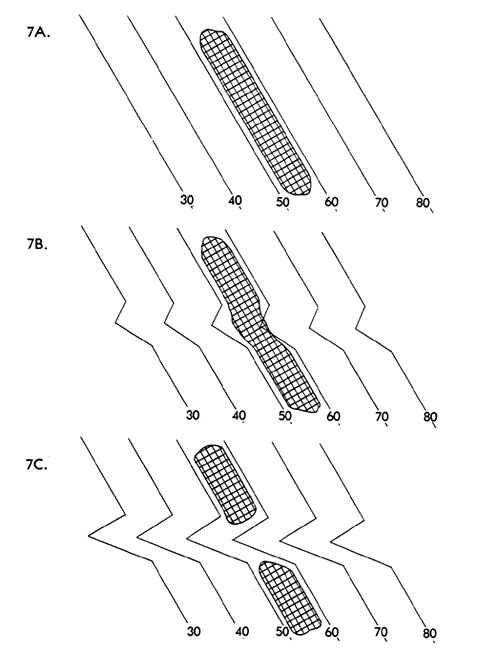
Figure 7. Disjunction of a species population range aligned along a stress field gradient by intervening climatic change. In 7A, the initial conditions are specified: an "elongated," R=0 population and a uniform gradient of stress. In 7B, climatic change has been locally initiated. In 7C, climatic change has been completed, leading to a disjunction. This disjunction may or may not persist, depending on subsequent events. Numbers labelling isolines indicate stress magnitude.

[[p. 145]] the gradient it is on (and thus cannot expand further downgradient), there should in theory be a tendency for it to move away from the higher stress area on the upgradient side. The result should be localization of the population along contour (this notion will also be relevant to the discussion on refugia, relicts, and altitudinal zonation to be presented later). This pattern of distribution will be most prevalent perpendicular to strong stress field gradients in areas of static climatic conditions. (Note that in this work, conditions such as these may be associated with the southeastern quarter of the study area. It was found that the lowest-K groups employed in this study, salamanders, frogs, and turtles, do show a slight but distinct elongation of the shape of their distributional ranges in this area; this was discovered while carrying out the set of tests described in Chapter VI). By attaining this range pattern, the population will be minimizing entropy with respect to its individual evolutionary potential (because it will be able to specialize with respect to a narrower range of community conditions: K selection (Pianka, 1970)), and maximizing entropy with respect to its contribution to the progression toward steady-state conditions (because such specialization will support a more regular pattern of spatial interaction and a more regular turnover rate of the materials it processes and returns to the environment). This is in effect a simple resource partitioning model (MacArthur, 1972).

    Given these initial conditions, let us now envision a rapid climatic change occurring in the area. The new conditions of the stress field topography are shown in Figure 7B. In Figure 7C, the expected distributional range response to the changed conditions is shown: the establishment of a disjunction. This disjunction will be viewed in retrospect as a vicariance event if and when the two population fragments [[p. 146]] produced drift genetically apart to a sufficient degree to become separate species (again, as some combination of initial differences in them and subsequent divergence events).

    The above scenario I will call for purposes of convenience an "active" vicariance event because it assumes a topographical change in the stress field over time as the forcing function for speciation. It is possible to imagine, however, a vicariance event in which there is no such change involved (a "passive" event). Instead, the activating force is a change in the K parameter inherent in a particular population.

    It would be convenient for vicariance studies and their posited corroborating method of constructing "geological cladograms" (a reconstruction of the way geological/climatological events tend to split up environments over time that is cast in the form of a dendrogram analogous to the cladograms describing phylogenetic affinities) if all vicariance events were ones in which local physical environment changes resulted in population bifurcations in space. Unfortunately, we cannot rule out the possibility that a static stress field topography might also take part in a vicariating episode. This theoretically could happen if: 1) the K parameter value associated with a given population changes (lowers); and 2) the stress field in the area is of heterogeneous topography. If the K parameter drops, regardless of immediate environmental/ecological influences, the result will still be contraction of range, since this will be the only way the population will maintain equilibrium conditions with its immediate biological/physical environment. Again, such contraction (resulting from local extirpation) will tend to take place first over highest stress areas, since it will be these that pose the most difficult conditions for meeting such equilibrium. Under the right topographical conditions, the result [[p. 147]] might be a separation of the population into two fragments in every other respect identical to the results of an active vicariance event. See the sequence of events diagrammed in Figure 8.

    What might cause such a lowering of the R parameter independent of local stress field circumstances? One possibility is the effects long-term change in atmospheric composition might have on physiological processes within the organism. Changes in, for example, the oxygen levels in the atmosphere over time might have led to direct extinction of many forms whose initially-evolved strategies of processing oxygen could not be adjusted to the handling of later higher levels. Related ideas concerning the impossibility of selective influences on certain vital adaptive structures within organisms are currently being developed as a part of the "molecular drive" hypothesis of evolution (Dover, 1982; Dover et al., 1982; Rose and Doolittle, 1983). Gould and Lewontin's (1979) arguments regarding general and cumulative constraints on the selection process are also relevant in this context, as here we must begin to consider that not all trade-offs balancing the maintenance of both a physiological steady-state and continuing ecological function are likely to be possible (and for reasons peculiar to the history of adaptational development in particular lineages). Early stages of an impending collapse in a population's thermodynamics would be interpreted here as a lowering of the population's K parameter (since it would involve a reduction in the population's potential range of interactions with its environment). Although inmost cases the resulting fragmentation of the population would simply represent the first step toward eventual extinction, it is possible that such fragmentation, coupled with the resulting re-assortment of gene pools and subsequent drift and mutations, might be enough to save the populations (that is, elevate the K

[[p. 148]]

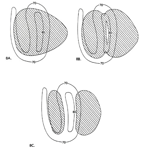
Figure 8. Disjunction of a species population range resulting from internal changes in population fitness. In 8A, the initial conditions of range and stress field topography are specified. In 8B, the K value associated with the population has begun to drop, causing range reduction. In 8C, the process has resulted in a disjunction. Numbers labelling isolines indicate stress magnitude.

[[p. 149]] parameter of each to a point permitting persistence).

    Such events might or might not be rare. In any case, resettings of the K parameter must be the rule in the "progressive" speciation process in general; were this not so, the history of life would indicate no progression toward forms capable of penetrating more and more harsh environmental conditions, while continuing to have large distributional ranges. The existence of this trend raises no special problems for the approach taken here; I have already suggested that the isolation of populations occasioned by a vicariance event is likely to lead to the production of two new species given differences in the gene pools of the two sister populations and the different sets of selection mechanisms in operation in each habitat they occupy. This view actually differs little from the present way vicariance-sympathetic biogeographers view the process of speciation (Eldredge and Cracraft, 1980; Wiley, 1981; Nelson and Platnick, 1981). Nonetheless, it suggests beyond the vicariance understanding some evolutionary relationships that seem worth exploring at this point.

    It has been stressed in this work that both the abiotic and biotic sectors are relevant to an understanding of the problems of biological distribution. Moreover, it has been accepted that the overall system is progressing toward steady-state conditions under which the exchange of materials back and forth across the abiotic/biotic interface constitutes some unchanging rate of turnover. Can these ideas be linked through the present model? More specifically, can we use the understanding presented here to interpret the long-term results of speciation processes as contributing to a system-wide state in which entropy production is eventually maximized?

    The production of maximum entropy in a biological community sense must [[p. 150]] be associated with the development of a highly diverse biotic sector, since it is through the joint material processing contributions of an array of specifically-adapted forms at a given location that the system will eventually reach a complexity and stability assuring constant turnover rates of all vital materials. In reality, such a state can never be reached at any one location, since irregular exogenous forces continually relegate community systems to sub-entropy-maximizing states. Nonetheless, we can still expect the "world community" system to reach such a state, since its long-term development is not a function of changing exogenous forces. This is true whether or not one believes that the pattern of evolution is affected by earth's occasional collisions with extraterrestrial debris (Alvarez et al., 1980); regardless, the earth is fundamentally a closed system with regard to mass transfer. The question we now ask is how we can evolve a system of organismal lines that produce the kind of diversity that ultimately functions in an ecological context to maintain maximum entropy production.

    The key problem here is how to imagine a dynamic equilibrium in which extinction and origination processes balance one another without loss of evolutionary information being involved. Because the environment does change, we must accordingly expect organisms to react in certain ways; for example, extinction. Under steady-state conditions, replacement (in some sense) of these forms is necessary to the continuation of the equilibrium state. Consistent with the ideas presented here, such a system might function in the following fashion.

    Let us first suppose that the ecosystem has in fact just reached that state wherein turnover rates of all material resources at the world level will remain constant, independent of the particular biological forms which [[p. 151]] mediate that structure. This does not mean that the production of new types has ceased; rather, that any such production has become irrelevant insofar as global material and energy cycling processes are concerned. Thus, a steady-state has developed with respect to energy exchange across the fundamental interfaces involved. Meanwhile, at the biological level, with its continuing turnover of populations, a true dynamic equilibrium is specified. With environmental conditions in a continual state of local flux, changing stress field topography will impose changes on the pattern of spatial interaction among biotic elements that include extinction and the isolation of segments of once-continuous populations from one another. Our intent now is to show how the two latter processes might take place under such steady-state conditions.

    Under these conditions, the biological system will be both as diverse as it can be (with regard to its mediation of spatial interaction processes, and not necessarily in terms of absolute diversity levels--note the relevant comments of E.P. Odum (1971) and Margalef (1968) regarding diversity levels and successional stage). Another way of putting this is to say that the world sum of K parameter values will be maximized, since some maximum amount of spatial interaction connected with processing energy and materials will be in operation.

    In a system proceeding toward the steady-state, emphasis must invariably be on radiative-type evolution initially; that is, toward divergence leading to minimum entropy production on a by-population basis. Feedback controls on such divergence will only be evident in the long-term sense by the way the overall system responds (through the nature--regularity of rate and volume--of turnover of processed materials). Major mutations/allelic recombinations may promote the development of major [[p. 152]] adaptive innovations resulting in greatly increased K parameter values for a population that signal further entropy minimizing at the population level, but such increases will only continue as long as the sum of all such innovations continues to refine material turnover characteristics in the system as a whole (see Conrad, 1983). Once the biotic sector reaches a state in which the sum of its component populations have refined such turnover characteristics to some unimprovable point, entropy will have been minimized ipso facto at the population level, and maximized at the ecosystem level (compare this view with the comments by Greer-Wootten presented in Chapter III). At that point, removals from the system (extinctions) will tend to be balanced by speciations, but there will be no net increase in system entropy production, and thus no further increase in the sum of K parameter values.

    Now if, because of extinction, a population disappears, the steady-state will be interrupted unless something happens to take up the slack. Two scenarios can be envisioned according to the thoughts presented here to satisfy the regeneration of equilibrium conditions.

    First, an environmental change-caused speciation event might take place. Open niches caused by an extinction might be filled through either sympatric or allopatric speciation, if a portion of another population inhabiting the same general area as the extinct form is cut off from the rest of its population by intervening climatic/environmental change (and, with the aid of its own genetic uniquenesses as a starting point, develops into a new species).

    The second means of equilibrium maintenance in the face of extinction devolves from strictly biological level considerations. Wherever a population becomes extinct, we should expect certain implications with [[p. 153]] regard to the remaining community structure. If other populations spatially interacted with the extinct one in any fashion (as is invariably the case), their own equilibrium will be disturbed. This will result in new, forced selection regimes (not drift, because past structures are irreversible), and a consequent lowering of K parameters associated with the populations responding. Such lowering will result in shrinking ranges, isolation of populations, and speciation of a type described earlier. The resulting re-definition of community interactions toward increasing localization of populations will mean a tendency toward the development of many low-K populations under these conditions, as opposed to the development of relatively fewer low-K populations under the climatic change scenario.

    These two scenarios ("type one" and "type two") may be geographically linked in the following fashion. First, faunas in areas of high climatic fluctuation (such as the temperate and high latitude zones) will tend to develop in a scenario one fashion, whereas faunas in areas of more stable climates will tend to follow the second one. Second, if we accept that evolution proceeds through divergence, within any given lineage we would expect early divergences to be more of the type one kind, and later ones to be more of the type two variety. This will occur because the novelty of a root form of a given lineage is synonymous with a K parameter elevation. This in turn indicates a trend toward generalization, high dispersability, and the ability to occupy a new range of habitat types (essentially, an r-selection regime: Pianka, 1970). The last characteristic especially is important, because it will mean such a population will tend to spread itself over a range of climatic conditions, and with natural variation in these over time, isolation (vicariance) events will occur.

    Another factor must be taken into account, however, to complete the [[p. 154]] understanding of the extinction-origination balance suggested here: the isolating factor inherent in dispersal into new areas. Fundamentally, dispersal in the view suggested here represents range expansion. This is inherent in the spatial evolution of range whenever a population represented by a certain K parameter at a given time is not representable as being in the R = 0 state at that same time. Dispersal is thus viewed simply as the mechanism which ultimately ensures a balance be obtained between adaptive potential and the enactment of that potential in contributing to the processing of biotic and abiotic resources inherent in the community structure within which it exists. It is the spatial reaction to the splitting of a gene pool and the associated disequilibrium generated.

    Given the preceding comments, we may proceed to the description of a general picture of the extinction-origination equilibrium as conceived here. Within particular lineages (and in general, for the sum of lineages) there is a trend over time for particular major evolutionary innovations to lead to explosive radiations--both with regard to the development of further lineages and to geographic expansion of range--and in general to operate under a type one vicariance-and dispersal-aided speciation regime. As various lines proceed toward their ultimate biological development, however, the evolutionary regime moves in the direction of type two conditions. (recall, also, that "active" vicariance events are involved in each--but not necessarily to the same extent--see below). The eventual interactive result of these two influences on general system evolution is an extinction-origination equilibrium: when certain populations fail as a result of chance events, their role in contributing to the overall equilibrium state is maintained by local speciation events. The nature of the latter will in large part be determined by the character of local [[p. 155]] environmental conditions; i.e., the ecological/historical stability of the ecosystem there.

    A couple of further remarks can be offered before returning a final time to vicariance events and then proceeding onward. The direct role of the stress field concept has not yet been integrated into the present discussion. It should be recalled that high-stress areas are supposed to have at least two major effects on the distribution of organisms: 1) a controlling influence on the (aspatial) direction of community evolution; i.e., by imposing constraints on the specific kinds of attributes that must be developed to underwrite particular patterns of spatial interaction; and 2) a tendency to slow the process of range change of populations within the area. These being so, and given the views presented in Chapter IV on the parameterization of range change, we should expect that low-stress areas will tend to be inhabited by large-ranged populations. This has already been discussed in the description of analysis seven in Chapter VI, and empirical results presented that sustain this prediction. Moreover, we know in general that most of the largest-ranged species, for example Canis lupus (gray wolf), Vulpes fulva (red fox), and Castor canadensis (beaver), are forms largely "restricted" to lower-stress areas (that is to say, the non-desert and non-rainforest parts of the earth). Such forms are successful generalists, species whose adaptational flexibility permits them to exist under a qualitative variety of low-stress conditions.

    There is an important point regarding the above situation and the evolutionary process as envisioned here that has not been emphasized yet. New populations that have identical K parameter values at their inception will tend toward expanding their range to equivalent degrees; the actual range in square miles obtained, however, will be a function both of that K [[p. 156]] parameter value and the local stress field conditions. Recall from the discussion in Chapter IV that high stress conditions will act upon a diffusing population by slowing it down; assimilation into the local community interaction matrix will require greater adaptive change. Thus, more specialization per diffused spatial-temporal unit is generated under high-stress conditions, a relationship that conserves the entropy of the system. This has already been suggested by the discussion in Chapter IV. Now, however, the long-term effect of the specialization/reduction-in-range size equivalency can be put into its broader context: the low-stress areas of the world are those in which are likely to originate the major biological innovations that will continue the trend toward system-wide entropy maximization. This will be so because the forms involved will be less specialized, and will continue to be less specialized, than forms existing under (and giving rise to new forms under) high stress conditions. Moreover, this evolutionary conservatism will have a spatial component in that it will be spread over a larger area (i.e., be associated with large-ranged forms), providing relatively more opportunities for local isolating events to take place involving the stock population. Naturally, the long-term stabilities of local climates will also have their countering effects; as it turns out, the low-stress areas of the world are not the most stable areas climatically. As a result, the tropical rainforest has the greatest standing biomass and diversity of any community type, but most of the forms found there are very highly specialized and at this point surely incapable of giving rise to radically new lineages. I would note at this point that this idea is supported by the fact that man, for example, is thought to have originated in habitats that would be relatively low stress zones.

    [[p. 157]] A second comment concerns a fulfilled prediction that can be deduced from the general understanding of a system approaching overall biotic-abiotic equilibrium. It has been noted by several sources that we seem to be either in a period of relatively little major biological innovation, or nearly have reached the end of this stage of biological history altogether. I support the latter idea. The approach to the steady-state would explain this pattern (and of the apparent approach toward constancy in numbers of orders in at least some groups: see the data of Sepkowski (1978) and Kurten (1971)); moreover it would also explain the curious fact that a number of the widest-spread mammalian genera (for example, Felis,Canis, and Lepus) each contain many species that can freely interbreed with one another. In these cases, I believe, the associated K parameter values are so high that further speciation into permanent new populations is extremely difficult. Simply, the adaptational suites of the species involved are so flexible as to be able to cope as is with community interaction structure regardless of underlying stress levels and how these fluctuate with time. With the exogenous control on the evolution of the system thus largely countered, further change will revert to a drift-like evolutionary regime, now emphasizing behavioral sophistication. The development of particular advanced behavioral capabilities will likely promote secondary structural level changes (in the same recursive fashion as that involving the biotic and abiotic sectors in general) which will be correlated with speciation events. Importantly, however, the new "species" resulting will remain as unspecialized as their immediate ancestors; i.e., genetic changes that have occurred will not represent an isolating factor at that level in that later re-introduction of bases through hybridization will have no effect on the developmental or physiological viability of the [[p. 158]] offspring (because they will have no impact on their ability to take part in spatial process). In short, the new "species" emerging will increasingly become no more than the chance product of drift associated with temporary physical isolations, and will easily be reabsorbable. This interpretation, by the way, can be extended with minimal logical difficulty to conditions of human and human cultural evolution as well, where the differences among peoples reduce to behavioral, and not genetic, causes.

    The relevance of the trends discussed to vicariance studies should be fairly apparent. For one thing, it suggests that high-K parameter populations will be poor subjects for vicariance-type analyses, as will low stress areas. Such conditions favor dispersal-oriented interpretations or vicariance-like situations which result in "behavioral synapomorphies" that may be harder to identify. So far, vicariance biogeographers have been finding this out on their own; almost all vicariance analyses are tropical in their geographic frame of reference, and I know of no vicariance interpretations for mammalian groups.

Adaptability and the "Adaptive Landscape"

    Though it might be complained that the remarks of the last section seem to have little connection to present directions of argument in theoretical biology, I believe that the differences are more apparent than they are real. The apparent differences stem from the fact that the present work represents an argument for a new kind of research program more than it does the extension of an already-established one. There is thus a lack of relevant literature at the empirical level that can be referred to to defend many specific points. Complicating the latter difficulty is the unwillingness here to resort to biological arguments to defend positions [[p. 159]] regarding distributional characteristics. Still, it should be noted before moving on to some more specific considerations that the general form of the argument is not so different from that used to describe in general biological terms the relation of adaptability to evolution.

    Conrad (1983: 216) has recently described the relationship of adaptability to classical views of the adaptive landscape. The latter can be portrayed as "a plot of fitness against gene frequencies.... In this picture of evolution....one sees the evolution process in terms of populations climbing the multidimensional hills and peaks in this landscape...."Conrad further develops his discussion after adding a third axis (environment) to his "landscape" and substituting nucleotide sequence for gene frequency (pp. 217-220):

"....The environment-parameterized landscape is a hypercloud of lines....If all the points in this hypercloud are connected by straight lines, the envelope of these lines becomes a fitness hypersurface, with multidimensional peaks and valleys.

    The fitness hypersurface has a global structure (the topography of the adaptive peaks and valleys) and a local structure which determines the ease with which particular peaks may be climbed by an evolving population....

    According to the bootstrap principle of evolutionary adaptability, populations will tend to move to regions of the landscape which are easily traversible, either because the pathways between peaks are smoother, because the peaks themselves are more climbable, or because there are peaks in the region....If a genetic variation moves a population to a region of the landscape which is more traversible, this variation will be drawn along with the evolutionary movement allowed by this increase in traversibility. Since any variation is a cost in terms of efficiency, a population must expend free energy to occupy a region of the landscape which is more amenable to evolutionary hill climbing. In effect, then, biological systems use free energy to increase the traversibility of the adaptive surface on which they are evolving....

    ....such a surface is occupied (in the real world) by many populations simultaneously climbing either the same or different peaks. Each such population is part of the environment of every [[p. 160]] other population. In principle this can be incorporated into the adaptive surface by introducing into the set of environmental axes a numbers axis for each possible genome sequence. Thus, as the numbers associated with each population change, each point on the surface will move, just as it would move as any environmental parameter changes. It might be pushed either higher or lower on a given peak, off a peak, or onto another peak. Since it is hardly reasonable that arbitrary shifting of a point along any of the environmental axes would push it uphill as often as it would push it downhill, a condition for the fitness of the various species represented on the surface to be nondecreasing is that the hills do not move relative to them faster than they can be climbed. This is an important point, for it means that selection for rate of evolution is not based solely on the advantages accruing to those species which can optimize more rapidly, but also on the disadvantage of de-optimization in those species which cannot keep pace with the relative motion of the landscape."

    The following observations can be made regarding the above passages:

    1) First, it is apparent that the concept of the adaptive landscape is not far removed from ideas presented here. Indeed, it is not too much to suggest that these simply represent different perspectives on a single process. Conrad provides a framework within which adaptive change within populations may be contextualized; in the present study, adaptive change is portrayed as a phenomenon that takes place across populations.

    2) In Conrad's simplest scenario, adaptive change is viewed as the "ascension" of peaks in the adaptive landscape. In the present context, this process is linked to entropy minimization, since adaptive change is viewed as the ends whereby spatial interaction becomes less variable with respect to controlling environmental conditions. Nonetheless, we should be careful not to jump to the conclusion that we can associate with any given population any particular peak of adaptation. Given the prior constraint of spatially-varying environmental stress and the spatial interaction characteristics demanded thereby, the notion of a peak in the adaptive landscape becomes more a function of geography than it does biology. [[p. 161]] Indeed, if this were not the case, we could scarcely understand the relationship of geographic isolation to speciation.

    3) One of the great disadvantages of Conrad's scheme is the interdependency of the axes defining the adaptive landscape. To make any sense out of the adaptive landscape device, it is necessary to erect a "fitness" axis which can be understood only in terms of the other two components of the system. While there is nothing wrong with this as an effort to depict system potentials, it does not in itself provide a clue as to the actual mechanism of change--in Conrad's terms, how "traversibility" of the system is increased. Conrad explains that "free energy" is used to effect such change, but how can this (truism) contribute to an improved geographical understanding of the meaning of this traversibility? Free energy may be defined as "the capacity of a system to perform work" (AGI, 1962: 195). Through the present model, such capacity may be stated in either biological or geographic terms; i.e., as the maintenance of the set of biophysical conditions associated with a particular pattern of spatial interaction. The free energy of a spatial configuration (e.g., organismal distribution) is easier to relate to possible future states than is that of a biological (i.e., genetic) configuration, however, because specification of such future states in the latter case necessitates an a priori understanding of fitness. Through the spatial interaction approach, fitness assumes meaning ipso facto: as presence/absence. A form is adaptively "fit" with respect to the conditions at a given location simply if it exists there. In the present model, the likelihood that a given population will exist at a given location is ultimately a function of local characteristics of the stress field and the population's overall adaptive flexibility and [[p. 162]] history. Fitness is thus viewed here as an epiphenomenon, since it is the result of the operation of the adaptive landscape rather than an element defining it. We still find--just as Conrad would have us believe--that increased traversibility yields increased fitness, but we must now view fitness as a kind of "compromise equilibrium" between biotic potential and environmental constraints. This is an appealing position, because it is better lent toward understanding how traversibility of the overall system is increased; i.e., through the refinement of spatial interaction patterns and attending increases in free energy supply.

    4) A final point may be made regarding the concept of the adaptive landscape and its relevance to zoogeographical studies. Conrad could well argue that I have been too hard on his model, as the environmental parameters that form a component of the adaptive landscape could theoretically be geographically compartmentalized in such a fashion as to account for the spatial interaction factor I describe here. This is true enough, but there seems no reason to go to such lengths. The result would be an impossibly complex description of system uniquenesses. It would seem more efficient to proceed in a different manner. If we can accept that evolutionary causal factors might be more directly approached through the study of spatial interaction patterns (i.e., the relationship of distribution to spatial variation in relevant aspects of the abiotic sector), expansion of the latter effort might increasingly set the stage for the testing of hypotheses regarding the spatial dynamics of more strictly biological phenomena. Although it is beyond the scope of the present work to attempt to detail the possibilities of the biological side of this endeavor, I have discussed here some aspects of the "distribution-as-spatial [[p. 163]] interaction" issue. Chapter VI was concerned largely with the testing of hypotheses regarding predicted patterns of distribution in a particular study area. The second section of this chapter consisted of some ideas on the causes of distribution pattern change over longer periods of time. In the next three sections, emphasis is placed on further means of bringing theory and empirical validation closer together.

The Analysis of Cumulative Pattern Development

    A fundamental idea underlying this work is that spatial interaction among the components of the earth's surface system leads to system evolution through an overall increase in efficiency of cycling of vital resources. This means that the mean level of stress of the overall stress field must have decreased through time. Such a general decrease must in of itself have an effect on the areas of distributional ranges, all other things being equal: a general increase in size. The easiest way to envision the dynamics suggested here is to first imagine a general stress field whose relative topography remains constant through time, but whose levels of stress decline uniformly in space through time. Populations will respond to this lowering through time by expanding their sphere of influence; i.e., the disequilibriun engendered by a reduction in cost of resources supplied will be met by a refinement of spatial interaction. (These remarks are predictable, since the recursive causal structure of the model entertained here necessitates them: the evolution in the biotic sector summarized as an increase in the sum of K parameter values must have its correlate in abiotic sector change, and this is given by reduction in stress levels.)

    These notions can be used to develop an interesting test of the ideas [[p. 164]] presented here. The test involves predicting what the distribution of population range sizes at given locations should look like under different circumstances of historical and ecological interaction. A related test was discussed in Chapter VI (analysis seven); here, however, we will generalize to a wider range of conditions. Let us first imagine a particular portion of the stress field topography upon which are distributed the ranges of some number of populations. The distribution of areas of these ranges is important to the discussion to follow. While in the real world we commonly find many species with small ranges and only a few with large ranges (MacArthur, 1972; Rapoport, 1982), this distribution must be considered to have evolved as the result of various constraints and opportunities (Rapoport, 1982). I should now like to re-interpret these constraints in light of present ideas. For this reason, we should envision our hypothetical portion of the stress field to be initially populated by a normal distribution of range sizes, and imagine how subsequent changes in the system might produce patterns mimicking real world conditions.

    We first allow our system to change through a uniform reduction in stress field magnitudes that does not affect the relative topography of the field. As before indicated, the overall result should be a general increase in range size among resident populations. If the range expansion is proportional to the K parameter value defining each population's range size, the result will be no change in the relative distribution of range sizes.

Note, however, that such uniform drops in the topography of stress might have important implications for the process of speciation. A relevant set of conditions is depicted in Figure 9. There, a low-K type population is first depicted in Figure 9A under R = 0 conditions. In Figure 9B, the magnitude of stress has been uniformly decreased, permitting an expansion of

[[p. 165]]

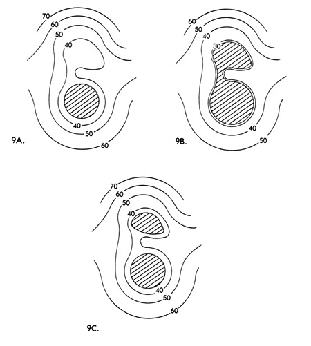
Figure 9. Disjunction of a species population range resulting from uniform changes in stress field topography. In 9A, the initial conditions of range and stress field topography are specified. In 9B, a uniform drop in stress magnitude has resulted in an expansion of range. In 9C, a return to original conditions has produced a disjunction, as in Figures 5 and 6. Numbers labelling isolines indicate stress magnitude.

[[p. 166]] range including a "spilling-over" into a new area. In Figure 9C, stress has temporarily increased to former levels, causing an isolation event as range sizes shrink in response to the change. If the isolation persists for a long enough period, the disjunction may result in biological as well as physical separation (i.e., allopatric speciation).

    Under such circumstances, therefore, we might expect a continuing increase in the relative proportion of small-ranging species. The reason is that large-ranging forms will tend to be less affected, as their adaptive flexibility will make them less subject to stress-induced disjunctions. As a result, the distribution of range sizes in such an area will tend to move away from a normal distribution and toward a negative exponential relationship.

    It is important to note, however, that similar results will not obtain where eco-geographic conditions vary greatly over time and/or where corridor conditions (Simpson, 1940) encourage a progression of introductions of wide-ranging forms to an area. Where climatic change is frequent, of considerable magnitude, and of relatively irregular nature, small-ranging populations will be at a disadvantage. Their general adaptive inflexibility will work against them, as the habitats to which they have become specialized may disappear quite rapidly, forcing them into extinction. One can view this in stress field terms as a rapidly changing topography requiring biological adjustments beyond the capability of small-ranging, highly inflexible forms. In an area characterized by these conditions we should expect the distribution of population range sizes of resident populations to be negatively skewed, as there will be "distributional selection" against small-ranging species. For highly-stressed areas (for example, deserts), we would expect a large percentage of species present to [[p. 167]] have medium-sized ranges, as the high stress levels would tend to prevent even very flexible forms from dispersing into the area from outside. For lowly-stressed areas, an expected influx of large-ranging forms would tend to increase both the skewness and the kurtosis of the distribution of resident population range sizes: more resident populations would have rather large ranges.

    These predictions are testable. Unfortunately, testing them requires data sets of a type that are not generally available. Nonetheless, I have been able to retrieve some relevant information, and this can now be discussed.

    The distribution data collected in the present study provide some indication of the validity of the discussion just presented. Although range sizes have been categorically ordered here for different purposes (per analysis seven of Chapter VI), these still can be used in the present context. First, we should summarize what patterns of distribution of range sizes we should expect under differing combinations of historical and ecological conditions.

    The projected patterns, per earlier discussion, are presented in Figure 10. Three independent variables are diagrammatically integrated: 1) length of ecological history of the location; 2) magnitude of stress at the location; and 3) degree of irregular fluctuation of ecogeographic conditions over time. The length of history condition can be further subdivided into situations: 1) where evolution of the system is imagined to begin with a controlled a priori distribution of population range sizes; and 2) where evolution of the system begins de novo; i.e., where a previously uninhabited location becomes available for occupation (for whatever reason: for example, because of glacial retreat). Combinations of these factors are

[[p. 168]]

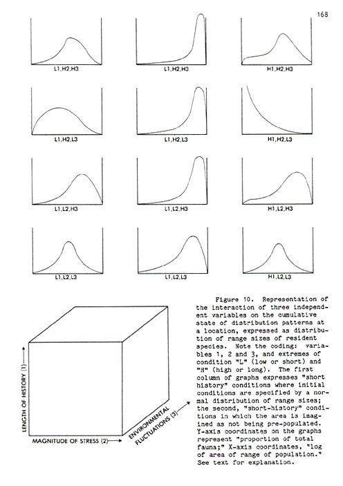
[[p. 169]] represented as twelve graphs in Figure 10.

    It would take too much space to discuss each of these sets of conditions in detail here, but a few items of importance can at least be pointed out. In general it can be stated that deviation from a normal distribution of range sizes becomes more severe with deviation from low stress and/or low fluctuation-in-stress conditions. Historical period of a given regime of conditions should also be strongly reflected in the distribution of range sizes. New environments (column two of the graphs in Figure 10) will all be characterized by a predominance of large-ranging forms, as such generalists will be the most likely forms to disperse into the area and will not have had time to differentiate in situ. (Note that this evaluation is consistent with the taxon cycle idea (Wilson, 1961; Ricklefs and Cox, 1972)) and with both succession theory and ideas on the dispersal abilities of r-selected forms: see Van Valen, 1971.) From this starting point, however, reaction to the local stress field will bring about different kinds of changes under different sets of conditions.

    (It must be admitted regarding Figure 10 that the relationships posited represent subjective assessments of the results likely under particular sets of conditions. Nonetheless, these should on the whole provide reasonable portrayals as long as one understands that present discussion on the subject is necessarily abbreviated, and that a more rigorous treatment can follow the initial identification of fundamental relationships (Levins, 1966).)

    The present study area does not contain examples of all the combinations of conditions portrayed in columns two and three of Figure 10. At least four sets of conditions, however, seem reasonably well represented, and examples of these were analyzed accordingly. The results are summarized in Figure 11. The four areas chosen for investigation consisted of squares

[[p. 170]]

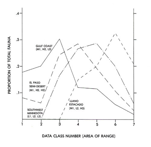
Figure 11. Comparison of faunal range sizes (ALLSPE) at four locations in the study area. Coding per Figure 10. See text for discussion.

[[p. 171]] of four grid cells centered on: 1) southwestern Minnesota; 2) the High Plains of Texas (the Llano Estacado); 3) a semi-desert region just west of El Paso, Texas; and 4) portions of the Gulf Coast of Mississippi, Alabama, and Florida and adjacent inland sections. These represent (per the classification of Figure 10), respectively, L1, L2, L3; M1, L2, H3; M1, H2, H3; and M1, H2, L3 conditions (where "M" designates an intermediate historical age). For each of these areas the number of mammals, reptiles and amphibians falling into each range size class were tallied and standardized into proportions. These proportions are graphed against size class in Figure 11.

    It is apparent that, despite the degree of subjectivity involved, the model described in this section does an excellent job of predicting the differences in distribution of range sizes among locations. The Minnesota location, a "new" environment opened with the retreat of the Wisconsinan glacier, is dominated by wide-ranging forms. The Gulf Coast location, a rather older, more stable, and more highly-stressed environment, is dominated by smaller-ranging forms. The semi-desert and Llano Estacado areas contrast as predicted. The latter is a low-stress area with a history of considerable environmental fluctuation (Wendorf, 1965); the former is also unstable, but at a higher stress level. As a result the latter has a more highly skewed distribution of range sizes: wide-ranging forms have been more able to disperse into it. Relevant pattern comparisons among the four areas may also be obtained by examining Appendices 2A, 2K, and 2L. (The patterns reported here, incidentally, also emerge when the distribution data are disaggregated to the level of the individual classes Mammalia, Reptilia, and Amphibia.)

    Rapoport (1982) has presented a graph charting the relative range sizes [[p. 172]] of over 900 species of birds in Africa. Unfortunately, his discussion does not include examples of location-specific distributions of range size. For Africa as a whole, however, the distribution is of negative exponential form. This brings up a point: the form of the curve representing distribution of range sizes must be scale-dependent. The larger the area involved, of course, the greater will be the bias of including relatively more small-ranging species.

    I have developed another data set whose patterns tend to reinforce the empirical findings just discussed. For approximately 1200 worldwide locations, I have computed a surrogate giving the distribution of range sizes of resident mammalian families. Although care needs to be exercised in working at the familial level in this instance (for example, because family range sizes are sometimes limited only by the total area of the earth), it is still fundamentally true that, like species, higher taxa may be viewed as having varying ranges of tolerance of environmental conditions. Allowing this, the patterns that emerge from this incompleted study fall largely into line with the predictions of Figure 10. For example, the most strongly positively-skewed distributions occur in the tropical rainforests of South America and Africa, the most negatively skewed distributions occur at high northern latitudes, and relatively unskewed and only slightly leptokurtic distributions characterize the major desert areas.

    The preceding discussion provides an explanation for some of the mediocre results described in Chapter VI. The failure of analysis eight, for example, can be traced (as anticipated in the discussion there) to mis-specification of cumulative historical influences. To check this, variable sets KSDCSMPi were added to the set of independent variables predicting the values of LIMRi. These representations of the recursive [[p. 173]] historical component in the development of present patterns were significant at alpha = .000 in four of the new regression models (REPSPE, TURSPE, AMPSPE, SALSPE) and at .050 in the rest (MAMSPE, LIZSPE, SNASPE, FRGSPE); the sign (positive) was correctly predicted in all. These are most encouraging results, as KSDCSMP is a very coarse surrogate (a better one could be constructed as a set of variables depicting, for each cell, the proportion of its fauna occupying different classes of range size).

    I believe that the areographic approach discussed here, given its basis in a more general ecological/evolutionary model, has considerable potential as a means of aiding biogeographic study. Its relationship to the earlier speculations of this chapter should be apparent: it provides a possible vehicle through which to separate ecological and historical components in the overall process of system change toward steady-state conditions. It should, for example, be a particularly useful tool for differentiating between the vicariance-and dispersal-dominated distribution regimes of different locations or, for that matter, associated with different lineages overlapping the same location. In such efforts, attention can be drawn not only to general spatial differences in patterns of range size distribution, but also to how these compare between the species level and higher taxonomic levels.

Altitudinal Zonation and Relict Populations

    Both of these topics have been popular subjects of discussion in biogeography for a long time. The earliest detailed altitudinal zonation studies were carried out by Humboldt at the turn of the nineteenth century; Merriam's work at the end of the nineteenth century, however, is probably the best known on the subject. The study of relict populations--especially [[p. 174]] of those found in tropical and temperate mountainous areas--also blossomed in the nineteenth century. Many of the early evolutionists, for example Darwin, Gray, Hooker, Lyell, and Wallace, were much interested in relicts, since they saw in them clues about the nature of both climatic and distributional change. It is interesting that altitudinal zonation and relicts are not usually studied in conjunction with one another; this probably devolves from the idea that the former is largely a subject of ecological interest whereas the latter is best understood within a historical perspective. Nonetheless, it should be apparent that zonation must be due to complex conditions of community evolution, and relicts may only exist in a given setting ecogeographic circumstances permitting. Here I should like to briefly consider the two phenomena from a somewhat more integrated starting position.

    Merriam's studies on altitudinal zonation (1890, 1894, 1898) were based largely on field work carried out in the San Francisco Mountains of central Arizona. His general conclusions on the matter were that temperature acts as the main limiting factor on vegetation; he then attempted to show how latitudinal variation in vegetation assemblages were mirrored in altitudinal assemblage types. His "life zones" concept eventually proved inadequate, but the fact remains that altitudinal vegetation gradients do in part mirror latitudinal changes.

    There are two likely ways historically that such zonation can develop. The hypotheses involved were argued over at great length by Darwin, Wallace, and others. One possibility is that zonation itself is a kind of relict structure. According to this view, large scale climatic changes such as those resulting from continental glaciation once forced species populations to unnaturally southern positions, where remnants remained in adjoining high [[p. 175]] altitude areas when climatic conditions reversed and the main body of the population returned to the north. Darwin (Marchant, 1916: 252) favored this view. A second view has it that high latitude forms might simply spread southward along the margins of mountain chains where they find appropriate microclimates (a position favored by Wallace: Marchant, 1916: 254-255). Undoubtedly both processes have been in operation to produce zonation in the midlatitudes, but note that neither really accounts for the zonation characteristics of tropical mountains, where many areas are populated by rather specialized forms not apparently related to higher latitude forms. True, there do exist isolated relicts of populations largely found to the north or south, but probably many or most of these can be accounted for by aerial dispersal.

    It is not difficult to apply the stress field concept developed here to an understanding of both zonation and relict populations evolution. As identified earlier, stress represents a constraining effect on biological organization imposed by abiotic sector resources that cross the abiotic-biotic sector interface at non-optimal rates. The spatial pattern of stress--that is, the topography of the stress field--is secondarily influenced by a multitude of general environmental/climatological factors, including surface elevation. Whereas the reliability of particular surrogates used to measure stress may vary under extremes of such influences, these per se have no bearing on the logical application of the stress concept to understanding the distribution characteristics of high relief areas. We should be able to interpret these in basically the same manner we would other areas.

    The altitudinal direction of the stress gradient must be a fundamental matter affecting the local distribution of organisms in mountainous areas. [[p. 176]] Tropical mountains, for example, are likely to exhibit a negative stress gradient from bottom to top, since tropical rainforests are very high-stress areas (but even this generalization will have exceptions, because stress values in some tropical mountain areas may be greatly inflated as a result of orographically-induced high precipitation levels and cool temperatures). Under such conditions, there will be a strong tendency for species populations to diffuse upslope, with highest K parameter forms moving the furthest. Once generally resident, such populations are likely to fragment and speciate according to local patterns of stress field topography, which may be very complex. The process imagined is roughly diagrammed in Figure 12. Since particular stress levels will be strongly aligned with particular elevational ranges and the overall gradient may be very steep, we would also expect a great deal of altitudinal separation of populations to occur (and thus a tendency for an elongated range patterns to evolve, for reasons similar to those discussed earlier), and zonation to result. The same kind of situation would be expected in midlatitude desert areas, where higher elevation is usually associated with cooler temperatures and more precipitation, and thus reduced stress.

    On the other hand, where neighboring lower altitude areas are low-stress in nature, increasing elevation may bring with it higher stress values, and a strong influence against the development of zonation. Such conditions are most likely to obtain in midlatitude and high latitude areas. There, only those populations characterized by very high-K parameter values will be likely to penetrate the upper slopes of the system (if they have originated from below).

    The major complicating influences to these scenarios are major climatic changes and the introduction of forms by means other than simple

[[p. 177]]

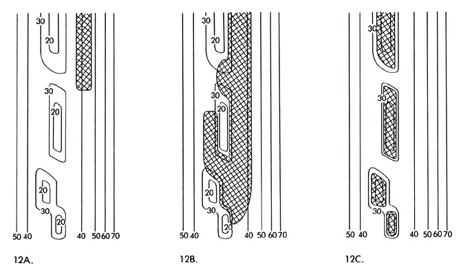
Figure 12. Schematic representation of an along-gradient dispersal event leading to the generation of relict populations. In 12A, the dispersing population has just reached the area. In 12B, it continues to disperse, probabilistically moving downgradient at the same time. In 12C, disjunction events of a type discussed earlier have occurred, producing relicts likely to persist in stable, low-stress environments (such as tropical mountains). Apparent examples of this process in action include speciation and subspeciation patterns of Sylvilagus, Bolitoglossa, and many other forms in the northern Andes (Muller, 1973; Hershkovitz, 1972). Numbers labelling isolines indicate stress magnitude.

[[p. 178]] marginal/upslope diffusion; e.g., through discontinuous aerial dispersal. During glacial periods, the shift of many population ranges southward would have introduced many new forms to the proximity of local topographical gradients. With the withdrawal of the glaciers and the onset of higher stress conditions at lower elevations in, for example, the southwestern United States, many populations would have withdrawn in two directions: upslope, and northward. Those segments that moved upslope might then become isolated as relicts if no continuous chain of satisfactory marginal environmental conditions kept them connected to the retreating main body of the population. The discontinuous dispersal influence is likely to be more relevant in the case of plants, whose seeds can be aerially dispersed directly or through the agency of birds.

    These principles might ultimately be applied to a consideration of the relative importance of the two major zonation-inducing historical frameworks discussed earlier in producing the conditions at a particular location. For the present, it will only be noted that spatial variation in zonation and relict population characteristics seems in a couple of instances to conform to the interpretation suggested here. In the United States, for example, zonation is much more pronounced on the southern side of the San Francisco Mountains than on the northern side, and on the western side of the Wasatch and Colorado Rockies than their eastern sides (as interpreted from even a casual glance at the "Potential Natural Vegetation" map compiled by Kuchler, 1966). In these cases, the greater degree of zonation corresponds with generally negative stress gradients; the lesser, with positive ones.

    The case of the Colorado Rockies is a particularly interesting one, since this area is thought to have been a major avenue for marginal dispersals during the glacial and interglacial periods. Such movement would [[p. 179]] be enhanced where altitudinal stress gradients were negative, since under these circumstances marginally-dispersing populations would be less likely to mix with those at lower altitudes. In general, in fact, one would expect positive gradient slopes to be "supplier" areas for marginal movement--but themselves to discourage such movement--whereas negative gradient areas would have the reverse properties. As a result, one would expect the latter areas to retain relicts, and the former not to do so. As a matter of fact, Weber (1965) has noted that the Rockies have an unusually small number of relict plant populations, as would be predicted here. My own data on mammals (and those of Hagmeier, 1966) also support this argument, since the spatial affinities of the mammals of the area are clearly more with northerly locations than they are with the High Plains to the east. Moreover, within the ten cells in the study area within and adjacent to the Colorado Rockies, thirty-seven per cent of the mountain species do not extend onto the Great Plains, whereas only six per cent of the lowland forms do not extend into the mountains. This is consistent with predictions, as the mountain forms are in general smaller-ranging (lower-K) forms and would be less expected to be able to conquer the stress gradient and occupy the lower altitude habitats.

A Regional Case Study

    One of the interesting tasks of zoogeography is accounting for locally-peculiar distribution characteristics. One such pattern is taken up in this section and interpreted in a fashion consistent with ideas that have already been developed. The object is to show that an internally consistent line of reasoning based in the model presented here might be used to gain an appreciation of the general causes of this pattern.

    [[p. 180]] It can be seen in Appendix 2A that the general area of the southeastern United States represents a very highly stressed area according to the present means of assessment. This quite large area centers on Tennessee and northern Mississippi and Alabama. Cool, wet winters and hot summers combine to produce yearly regimes including both surplus and deficit conditions, with the former being especially severe. This pattern has been in existence for some 5000 years (Delcourt, 1979; Solomon et al., 1980), apparently becoming accentuated by an increase in influence of Gulf of Mexico air masses. The stability over time is emphasized by palynological studies (Delcourt, 1979; Solomon et al., 1980) indicating relative constancy in the vegetation over the period, which postdates the changes that occurred in the immediate post-glacial.

    The southeastern United States has long been considered a refugium that operated throughout the glacial epoch (Wallace, 1880; Adams, 1902, 1905). With the final withdrawal of glacial ice, northern forms such as spruce retreated from Tennessee and other nearby areas to their present location. Note that such dispersal generates no problems of interpretation for the model presented here. Community conditions within such refugia probably operated under somewhat higher stress conditions than would have existed in more northerly habitats (if present patterns of relatively low stress in more northern locations are any evidence) had these been open. Retreat of the glaciers would have been accompanied by the evolution of a relatively gentle downgradient of stress that could have been easily followed, especially by generalist forms (i.e, both low stress and low gradient conditions would have been in operation).

    Beginning several thousand years ago, the stress conditions in the Southeast probably increased considerably, creating the development of a [[p. 181]] rather severe stress gradient away from the local high in the Tennessee-Mississippi-Alabama area (see Appendix 2B). This extends outward in all directions. According to the model presented here, we would expect populations in the area to tend to respond in certain ways to its influence. These should be all the more apparent, because of the severity of the gradient involved.

    One pattern that should be evident is that of "center-fleeing." Given that populations will tend to extend their range in the direction of lower stress conditions and that an increase in stress at a location should tend to fragment populations (ideas discussed earlier), we should expect to find evidence that the area in question is a center of dispersal of populations. Good evidence for this emerges from the present study. A number of polytypic genera ranging in the study area do in fact seem to have the Tennessee-Mississippi-Alabama area as their centers of distribution. I have included maps of four of these in particular in Appendix 4. Some commentary on these is helpful at this point.

    The four examples I have chosen are the reptile genera Natrix (water snakes) and Eumeces (skinks), and the amphibian genera Rana (true frogs) and Hyla (tree frogs). Appendix 4 contains both the individual species range maps for each genus and a composite map summarizing geographic variation in the total diversity of species for each genus. The composite maps especially show a tendency for low diversity over the highest stress area (which would not be predicted if this were simply a "center of endemism"), highest diversity in a (to one degree or another discontinuous) ring around this area, and a gradual decay in diversity beyond this ring. The pattern is especially obvious in Natrix and Rana. The interpretation consistent with the model presented here is that these populations have dispersed [[p. 182]] outward from their glacial refugium center over the last several thousand years, with the pattern and rate of such dispersal being strongly influenced by the development of the Tennessee-Mississippi-Alabama high stress area. Other polytypic genera (such as Bufo, Ambystoma, Desmognathus, Plethodon, Eurycea, and Graptemys) seem to exhibit a similar pattern. So do freshwater fishes (per data presented recently in a paper by McAllister and Schueler, 1983).

    Figure 13 provides some further information. In this is depicted the pattern of small-ranging salamander populations (per empirical analysis eight). Note the very strong "ringing" effect around the Tennessee-Mississippi-Alabama area. My interpretation of this is again that it represents a fragmentation process combined with the inability of these low-K forms to disperse very far down the steep stress gradient.

    Missing from the above examples are mammalian examples. This, however, we might expect, since mammal species are in general high-K parameter forms that would be less dominated by the gradient. Moreover, there are fewer polytypic genera of mammals that can be associated solely with the southeastern glacial refugium.

    We should also expect to find evidence of highly stressed low-K parameter individual species populations in the area. Such evidence would come in the form of populations in the process of fragmenting; i.e, vicariance/disjunction events. Examples of what I interpret to be as such are given in Figure 14. The coal skink, Eumeces anthracinus, is an excellent case, with disjunct subpopulations ringing the highest stress area and a few relict populations remaining within it. The distribution of the bullsnake, Pituophis melanoleucus, provides a good instance of the effect of the stress field topography in maintaining separation of subspecies

[[p. 183]]

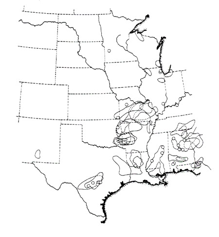
Figure 13. Small-ranging (less than 50000 square miles) salamander populations within the study area. Data from Conant (1975).

[[p. 184]]

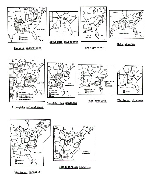
Figure 14. Range fragmentations theoretically referable to the southeastern United States stress maximum. See text for discussion.

[[p. 185]] populations. Ambystoma talpoideum, Hyla gratiosa, and Hyla cinerea are cases similar to Eumeces anthracinus, whereas Pseudotriton montanus, Rana areolata, and Plethodon cinereus are cases analogous to Pituophis melanoleucus. Fragmentation is also evident in Plethodon dorsalis and Hemidactylium scutatum.

    In the description of analysis seven in Chapter VI it was suggested that high-stress areas should be characterized by faunas of low mean cosmopolitanism and high standard deviations thereof. A review of the data I have collected suggests that this description fits the area in question here. Moreover, the center of the area is one containing relatively few boundaries (as can be seen in the example given in Appendix 2H), suggesting it to be a center of distribution patterns.

    The sharp ridge of high stress found in the area and the gradient emanating from it suggest in general the likelihood of a profound influence on gene flow in the area. This will likely affect the geographical distribution of subspeciation and phenotypic expression. Certainly, an examination of the distribution maps in Hall (1981) and Conant (1975) indicates that subspeciation in the area is of great complexity. A full attempt to confirm this prediction is, however, beyond the range of present purpose.

    A further expectation regarding distributional patterns in the area revolves around the notion that the stress field concept may be applied to the interpretation of community structures. There are a number of ways of looking at this; I will note but one here. In the past there have been a number of attempts to identify ecological units through the study of the distribution patterns of particular higher taxa (see as examples Webb, 1950; Hagmeier and Stults, 1960. Hagmeier (1966) performed an analysis in which [[p. 186]] he clustered data of a type similar to those collected here for mammal species into a set of "mammalian ecoregions." If in fact the model presented here is applicable, I would expect such ecoregions to bear a correlative spatial relationship to the stress field topography involved. This should be especially strong where gradients are high, since these are the places where direction of range change would ostensibly be most controlled. Hagmeier's maps (Figure 15) do indeed indicate provinces whose boundaries tend to parallel the contours of the stress field in the southeastern United States. Such patterns are likely the result of the tendency of down-gradient diffusing populations to spread sideways (along contour) as they change, range (again, the elongation effect discussed earlier), with the result that affinities among faunas will be greater along contour than perpendicular to it.

    Lastly, I will note again that there is some evidence that the "elongation" effect operates on a rather large scale across this particular area, and especially in the low-K parameter groups (turtles, frogs, and salamanders).

Simulation Studies

    The last subject taken up in this chapter concerns what is probably ultimately the best means of exploring the potential of the present model to deal with process studies: simulation. Simulation methods have not, to my knowledge, been applied to continental-level biogeographical studies involving a strong historical component. The reason is undoubtedly that simulation attempts must be grounded in relationship definitions that can be parameterized, and biogeography does not have a history characterized by the development of these kinds of concepts. The link to innovation diffusion

[[p. 187]]

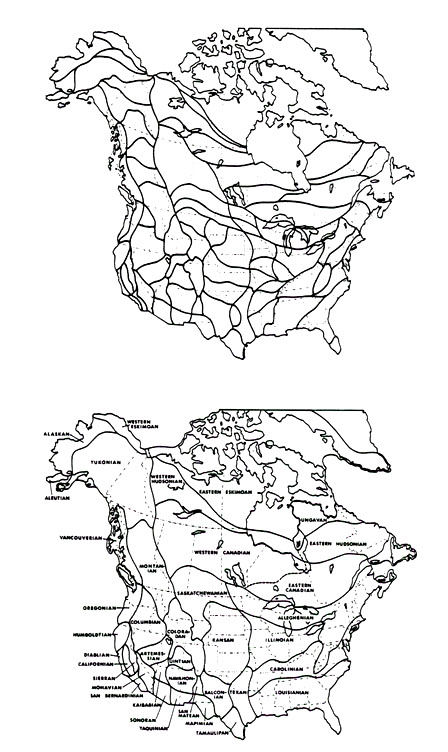
Figure 15. Mammalian faunal regions of North America (Hagmeier, 1966). The upper map portrays the fundamental units; the lower, their combination into provinces following a clustering operation.

[[p. 188]] modelling inherent in the present model of distributional dynamics, however, provides the flexibility required for simulation approaches (Brown, 1981; Hägerstrand, 1965; 1967).

    Although I earlier rejected the use of simulation in the present study, the decision involved was one of priorities and convenience rather than advisability. I believe the future development of the model proposed here lies in three distinct, but wholly complementary, directions. First, continued examination of state-space conditions aided by deterministic tests such as the ones employed here should be carried out. Many more predictions concerning the state-space relation of distribution patterns to the stress field forcing function should be possible; moreover, hypothesis-testing under the assumption of immediate types of control is relatively uncomplicated. Even more important should be attempts to apply the logic of the model to predictions regarding the nature of cumulative influences on distribution patterns. Such tests will be more difficult (less controllable), but will potentially extend the connection of the model to evolutionary process. In addition to such general studies, analyses of situational conditions should be carried out in an effort to determine whether particular locational ecologies and histories can be reconciled with the notion of the stress field causal factor. Two particularly good subjects for study would seemingly be the altitudinal zonation phenomenon, and refugium dynamics.

    A second area of study must be the refinement of the stress concept itself, and how it can be most usefully measured. I do not claim that the specific means employed here to measure stress cannot be improved upon; indeed, many other approaches seem possible. I used what I did largely because I felt that it was the simplest formulation that seemed likely to [[p. 189]] produce results within an empirical context.

    Once we have at hand enough descriptive information concerning distribution patterns of a type useful to a consideration of the state-space and/or historical predictions of the model presented here, we should be able to proceed to the third step: diffusion simulations. These will be used to produce artificial patterns whose measureable characteristics will parallel, hopefully, those of real world conditions. This will not be easy, because there will be several parameters involved, and it may be necessary to experiment considerably before results are obtained that can justifiably be compared to real world conditions.

    Nonetheless, once preliminaries are dealt with, it should be possible to study a rather wide range of phenomena, and these need not be limited to simple distributional pattern analyses. A necessary feature of the approach described here is the relation between adaptation and range change; it will be recalled that it has been postulated that the slowing of a range expansion front should be associated with an increase in specialization (a trade-off that maintains the dynamic equilibrium between population and physical environment). It should be possible to build into a simulation design the "memory" needed to keep track of adaptational change over space as the diffusion process proceeds. This opens up a host of possibilities for analysis at the biological level that can be compared to the purely spatial proceedings of the process. For example, the several kinds of speciation processes (as well summarized by Endler, 1977) now considered as possible might be investigated in more detail. As an extension, once the relation of taxon-specific parameter values is better understood, the relative importance of these processes for particular groups could be better investigated (both in terms of their purely spatial expression as [[p. 190]] distribution patterns and their associated impact on kinds of phenotypic expression).

[[p. 191]] APPENDIX 1: DESCRIPTION OF VARIABLES USED IN THE EMPIRICAL STUDIES

Introduction

    The variables described below are organized into three groups, per discussion in the text (Chapters V and VI). All values assigned to each variable were associated with a corresponding cell in the geographic sampling grid (see Figure 3). For most of the variables, this meant a total of 306 such values. For various reasons, however, some variables were composed of fewer than 306 values (for example, where secondary transformations of the distribution data resulted in division by zero and where the taking of spatial derivatives would have necessitated knowledge of conditions outside the study area).

I. Site Factor Variables

    The probable effect on distribution characteristics of a number of environmental variables exogenous to the present model had to be removed before tests could be applied. The variables considered were:

    XLAT: The latitude at the center of each cell (a surrogate for total energy available to the system).

    XMALT: The mean altitude in each cell. The geographic sampling grid was first laid over a USGS 1:7,500,000 scale topographic map that included the study area. Within each cell a systematic sample of nine altitudes was then collected; from each set of nine values the average was calculated.

    XSDALT: The standard deviation of altitudes in each cell (from the same sample as XMALT). Mapped in Appendix 2F.

    XRALT: The range of altitudes in each cell. This was assessed visually directly from the topographic map. XMALT, XSDALT, and XRALT were used to account for the independent effect environmental complexity due to altitudinal variation might have on distribution tallies.

    XOCLAK: The proportion of the cell falling within one cell's width (approximately 70.7 miles) of the Gulf of Mexico or the Great Lakes. XOCLAK was used to help account for possible biases in diversity and range boundary tallies associated with the more limited directional traversibility of the locations.

    XRIV1: The proportion of each cell falling within one-half cell's width (approximately 35.35 miles) of a river having a flow at that point of 15000 cubic feet per second or more. Mapped in Appendix 2G.

    XRIV2: The proportion of each cell falling within one-half cell's width of a river of total length exceeding 650 miles (in those parts of such a river where flow exceeds 500 cubic feet per second or is one-half or more of its highest flow if this is less than 500 cubic feet per second). Mapped in Appendix 2G.

    [[p. 192]] XRIV3: The number of river segments (per Horton, 1945) in each cell (of either XRIV1 or XRIV2 type) occurring within a circle of 150 miles diameter whose center is the center of the cell. XRIV1, XRIV2, and XRIV3 were used to help account for barrier effects imposed by rivers. The measures employed are arbitrary, but designed to help account for different possible interpretations of rivers as barriers (i.e., as representing environmental "areas" physically difficult to successfully cross, geomorphic influences on movement, and habitat partitioning influences).

II. Stress Field Variables

    As discussed in Chapters V and VI, measurement of stress field variables began with the construction of an isoline map of stress values derived from the climatological data base of 566 stations in the study area. The sample grid system of 306 cells was then superimposed on this map and various measurements made on a by-cell basis. The variables constructed in this fashion were:

    ZMSTRS: The mean value of stress in each cell. This was estimated from a systematic sample of nine values within each cell (as for XMALT). Mapped in Appendix 2A.

    Z1: The mean difference between the mean stress (ZMSTRS) in each cell and the mean stress values of the eight cells geographically surrounding it (a measure of local "unevenness" of the stress field).

    Z2: The standard deviation of stress values in each cell (from the same sample as ZMSTRS).

    Z3: The range of stress values in each cell (the number of mapped data classes present in the cell).

    Z4: The mean difference between each cell's Z1 value and the Z1 values of the four cells contiguous to it (a measure of local spatial change in unevenness of the stress field).

    Z5: The spatial derivative (slope or gradient) of stress across each cell (Tobler, 1970), using the values of stress at the midpoint of each segment of cell boundary as the basis for calculations.

    Z6: The spatial derivative of stress across each cell (Tobler, 1970), using the ZMSTRS of cells to the north, south, east, and west as the basis for calculations.

    Z7: The spatial derivative of stress across each cell (Tobler, 1970), using the ZMSTRS of cells to the northeast, northwest, southeast, and southwest as the basis for calculations.

    Z8: The mean of Z6 x 1.26 and Z7 (a standardized average of these two spatial derivative measures).

    Z9: The proportion of each cell perimeter that has a lower stress value than the mean stress (ZMSTRS) of the cell (a measure of local concavity/convexity of the stress field).

    [[p. 193]] Z10: The proportion of the circumference of a circle of 150 miles diameter centered on each cell that has a lower stress value than the mean stress (ZMSTRS) of the cell (a measure of local concavity/convexity of the stress field).

    Z11: ZMSTRS minus the mean of a systematic sample of eight stress values taken along the boundary of each cell (a measure of local concavity/convexity of the stress field).

    Z12: ZMSTRS minus the mean of the ZMSTRS values of cells to the north, south, east, and west of each cell (a measure of local concavity/convexity of the stress field).

    ZCGRAD: The spatial derivative of the spatial derivative (change in slope) of stress across each cell, using the Z8 values of cells to the north, south, east, and west as the basis for calculations. Mapped in Appendix 2C.

    ZGRAD: A principal component integrating the effects of Z6, Z7, and Z8 to form a general measure of slope, or gradient, of stress across each cell. The unrotated factor loadings of each variable on the component are on the order of r = .85. Mapped in Appendix 2B.

    ZRSTRS: A principal component integrating the effects of Z6, Z7, and Z8 to form a general measure of range of stress values within each cell. The unrotated factor loadings of each variable on the component are on the order of r = .85. Mapped in Appendix 2D.

    ZCONCV: A principal component integrating the effects of Z9, Z10, Z11, and Z12 to form a general measure of local concavity/convexity of the stress field (with respect to each cell). The unrotated factor loadings of each variable on the component are on the order of r = .80. Mapped in Appendix 2E.

III. Distribution Variables

    The basic data collected to generate the distribution variables consisted of presence/absence recordings of species, genera, and families is amphibians, reptiles, and mammals on a by-cell basis. These data were augmented by analogous recordings of range boundary presence/absence. Secondary transformations of these primary data followed.

    The distributional variables were named in a two-step process. A name was first assigned each variable type, independent of the particular organismal groupings that were studied with respect to that variable. The organismal groupings were then coded and referred to each variable. The organismal grouping codings were: AMP (amphibians), SAL (non-anuran amphibians), FRG (frogs and toads), REP (reptiles), TUR (turtles), LIZ (lizards), SNA (snakes), MAM (mammals), and ALL (amphibians + reptiles + mammals). The taxonomic level codings were: SPE (species), GEN (genus), and FAM (family). "AMPSPE" thus refers to the organismal grouping of amphibian species distributional ranges.

    [[p. 194]] In the descriptions to follow, the particular organismal groupings that were actually used in the empirical tests concerning each variable are coded as numbers to save space. The coding, followed by the total number of forms included in each grouping, is as follows: AMPSPE (1): 114; AMPGEN (2): 31; AMPFAM (3): 14; SALSPE (4): 57; SALGEN (5): 17; SALFAM (6): 7; FRGSPE (7 ): 57; FRGGEN (8): 14; FRGFAM (9): 7; REPSPE (10): 168; REPGEN (11): 64; REPFAM (12): 16; TURSPE (13): 38; TURGEN (14): 14; TURFAM (15): 6; LIZSPE (16): 47; LIZGEN (17): 13; LIZFAM (18): 5; SNASPE (19): 83; SNAGEN (20): 37; SNAFAM (21): 5; MAMSPE (22): 205; MAMGEN (23): 88; MAMFAM (24): 27; ALLSPE (25): 487; ALLGEN (26): 183; ALLFAM (27): 57.

    The distribution variables constructed were as follows:

    BDIV(1-27): The number of forms present in each cell ("total diversity"); i.e., each case represents a cell-specific total. BDIV25 is mapped in Appendix 2Q.

    BBOUN(1-27): The number of distributional range boundaries present in each cell; i.e., each case represents a cell-specific total. BBOUN25 is mapped in Appendix 2H.

    AVECN(1,4,7,10,13,16,19,22,25): The number of north-facing boundary vectors in each cell; i.e., each case represents a cell-specific total. A "north-facing boundary vector" was counted where a particular cell included within the range of a given form bordered a cell to its north which was not so included. AVECN25 is mapped in Appendix 2M.

    AVECS(1,4,7,10,13,16,19,22,25): The number of south-facing boundary vectors in each cell. AVECS25 is mapped in Appendix 2N.

    AVECE(1,4,7,10,13,16,19,22,25): The number of east-facing boundary vectors in each cell. AVECE25 is mapped in Appendix 20.

    AVECW(1,4,7,10,13,16,19,22,25): The number of west-facing boundary vectors in each cell. AVECW25 is mapped in Appendix 2P.

    LIMR(1,4,7,10,13,16,19,22,25): The number of continuous distributional ranges of 50000 square miles or less present in each cell; i.e., each case represents a cell-specific total.

    ECORR(1-4,7,10-13,16,19,22-24): For each cell, a correlation coefficient stating the relationship between the eight elements of sets "A" and "B", where set "A" = the absolute values of the differences between the cell's mean stress (ZMSTRS) and that of each of its immediate neighbors, and set "B" = the corresponding faunal association values between the cell and its neighbors.

    EECORR(25): The same as for ECORR, but with stress gradient values (ZGRAD) substituted for ZMSTRS.

    ESDEV(1-4,7,10-13,16,19,22-24): For each cell, the standard deviation of the faunal association values between the cell and its eight immediate neighbors. ESDEV22 is mapped in Appendix 2I.

    [[p. 195]] EDIF(1-4,7,10-13,16,19,22-27): For each cell, the difference between the cell's total diversity (BDIVi) and the mean of the faunal association values between the cell and its eight immediate neighbors. EDIF25 is mapped in Appendix 2J.

    KMCSMP(1,4,7,10,13,16,19,22): For each cell, a score indicating the mean cosmopolitanism of the species (on a by-group basis) present there (as described in the text). Cells populated on the whole by wide-ranging species have high scores, and vice versa. KMCSMP22 is mapped in Appendix 2K.

    KSDCSMP(1,4,7,10,13,16,19,22): For each cell, the standard deviation of the set of values also yielding KMCSMPi values. Cells populated by both small- and wide-ranging species have high standard deviations, and vice versa. KSDCSMP22 is mapped in Appendix 2L.

    CDIFDIR(1,4,7,10,13,16,19,22): For each cell, the difference in degrees between the compass direction of stress field gradient and the circular mean to cell centroid (see text) of AVECNi, AVECSi, AVECEi, and AVECWi values associated with the cell.

    CCIRVAR(1,4,7,10,13,16,19,22): For each cell, the circular variance (see text) of the AVECNi, AVECSi, AVECEi, and AVECWi values associated with the cell (a measure of the degree to which boundary vectors are not directionally uniform).

    CVAR(1,4,7,10,13,16,19,22): For each cell, the standard deviation of the AVECNi, AVECSi, AVECEi, and AVECWi values associated with the cell.

[[p. 196]] APPENDIX 2: SAMPLE MAPS OF VARIABLES USED IN THE EMPIRICAL STUDIES

Introduction

    In Appendices 2A through 2Q are mapped a sample of the variable sets employed in the empirical studies in this work. Space limitations preclude a mapping of all variable sets. With the exception of 2G, all the maps are isoline maps in which class shading becomes darker with higher values. Each map portrays twelve classes of data. The maps were produced through the routine F-MAP of the SYMAP package (Dougenik and Sheehan, 1979).

    To enhance the readability of the maps, index contours (darkened lines) are used to accent isolines separating the fourth and fifth, and eighth and ninth, data classes. Darkened lines also delimit the portion of the study area (usually all of it) that pertains to each variable set.

[[p. 197]]

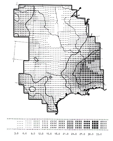
Appendix 2A. ZMSTRS (mean stress). The map is derived from the mean stress values of the 306 grid cells, not the original data. Values are dimensionless.

[[p. 198]]

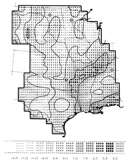
Appendix 2B. ZGRAD (local stress gradient). Values are dimensionless.

[[p. 199]]

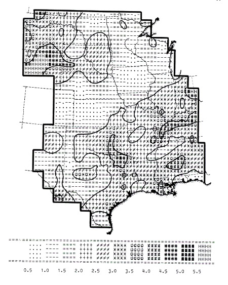
Appendix 2C. ZCGRAD (local change in stress gradient). Values are dimensionless.

[[p. 200]]

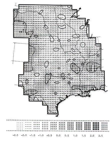
Appendix 2D. ZRSTRS (local range in stress values). Values are dimensionless.

[[p. 201]]

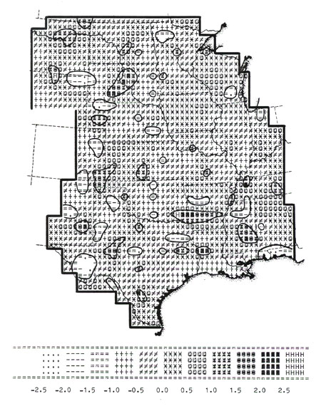
Appendix 2E. ZCONCV (local concavity/convexity of stress field). Higher values indicate greater convexity; lower values, greater concavity. Values are dimensionless.

[[p. 202]]

Appendix 2F. XSDALT (local standard deviation of altitudes). Values are in units of thousands of feet.

[[p. 203]]

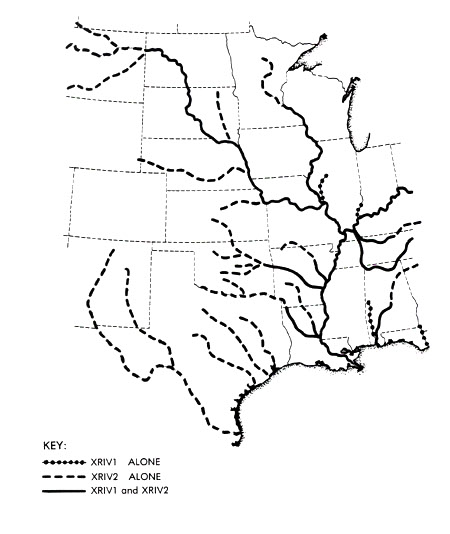
Appendix 2G. Location of the river sections associated with XRIV1 and XRIV2.

[[p. 204]]

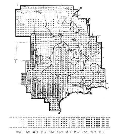
Appendix 2H. BBOUN25 (number of range boundaries present, ALLSPE).

[[p. 205]]

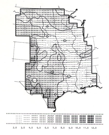
Appendix 2I. ESDEV22 (MAMSPE). See Appendix 1 for description of this variable. Values are dimensionless.

[[p. 206]]

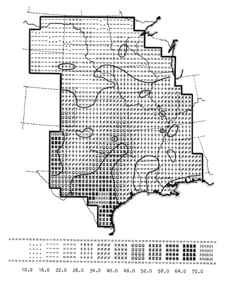
Appendix 2J. EDIF25 (ALLSPE). See Appendix 1 for description of this variable. Values are dimensionless.

[[p. 207]]

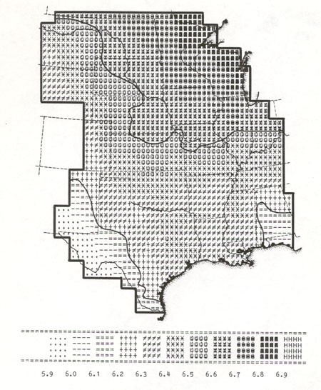
Appendix 2K. KMCSMP22 (MAMSPE). See Appendix 1 and Chapter Six for description of this variable. Values are dimensionless.

[[p. 208]]

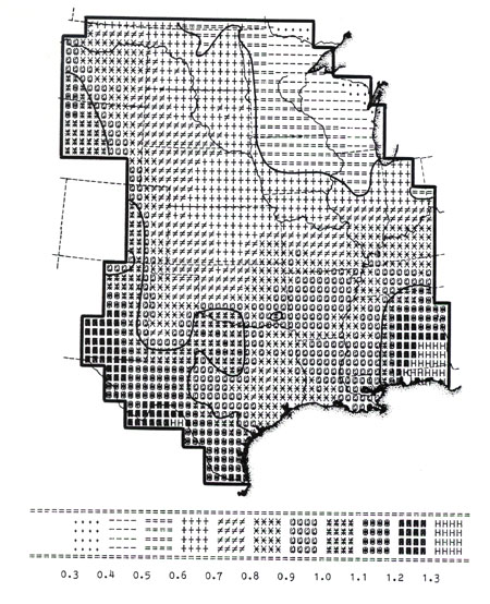
Appendix 2L. KSDCSMP22 (MAMSPE). See Appendix 1 and Chapter Six for description of this variable. Values are dimensionless.

[[p. 209]]

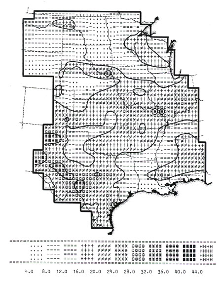
Appendix 2M. AVECN25 (ALLSPE). See Appendix 1 for description of this variable. Values represent total number of vectors.

[[p. 210]]

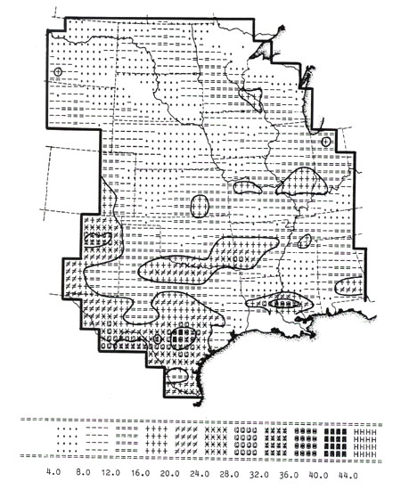
Appendix 2N. AVECS25 (ALLSPE). See Appendix 1 for description of this variable. Values represent total number of vectors.

[[p. 211]]

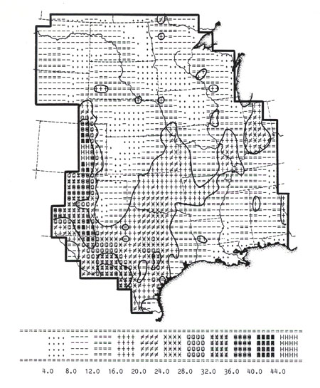
Appendix 2O. AVECE25 (ALLSPE). See Appendix 1 for description of this variable. Values represent total number of vectors.

[[p. 212]]

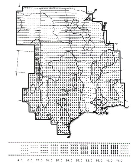
Appendix 2P. AVECW25 (ALLSPE). See Appendix 1 for description of this variable. Values represent total number of vectors.

[[p. 213]]

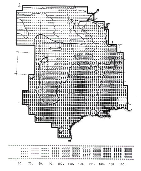
Appendix 2Q. BDIV25 (number of species present, MAMSPE).

[[p. 214]]

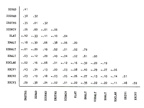
APPENDIX 3: CORRELATION MATRIX OF THE PRIMARY INDEPENDENT VARIABLES USED IN THE STUDY

[[p. 215]]

APPENDIX 4: DISTRIBUTION CHARACTERISTICS IN THE STUDY AREA OF FOUR GENERA OF HERPTILES:
RANA, HYLA, NATRIX, AND EUMECES

    In Appendices 4A through 4D are portrayed the distribution characteristics in the study area of species in four genera whose centers of distribution are roughly the southeastern portion of the area. Both the individual range maps of each species and a composite map expressing distribution of numbers of species are included for each genus. The data for the composite maps were taken from species distribution maps in Conant (1975); the latter are also reproduced here.

[[p. 216]]

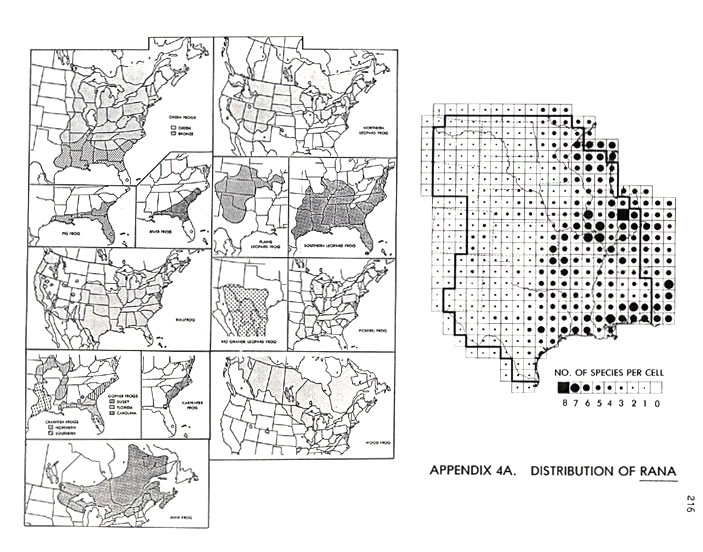
[[p. 217]]

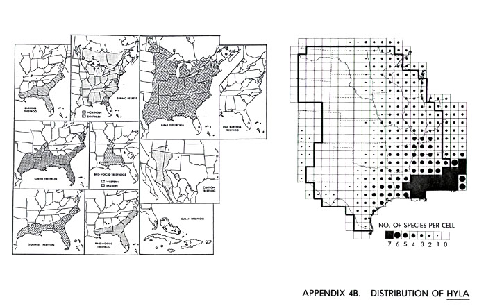
[[p. 218]]

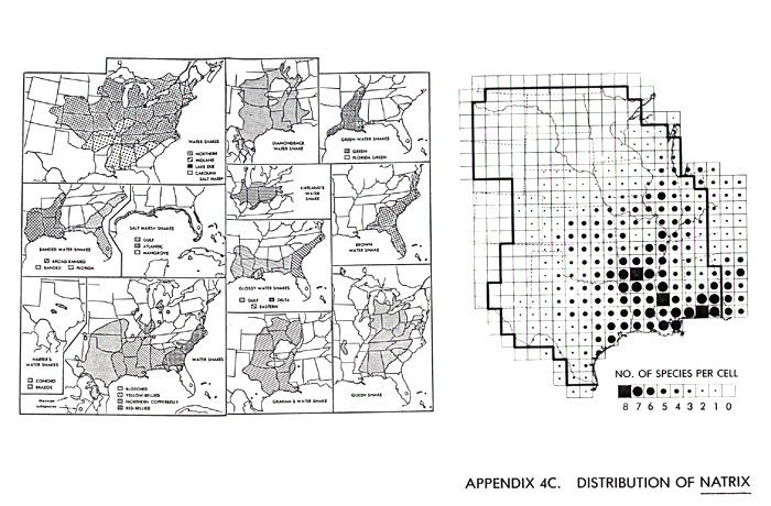
[[p. 219]]

[[p. 220]]

REFERENCES CITED

AGI (American Geological Institute), 1962. Dictionary of Geological Terms. Doubleday & Co., Inc., Garden City, New York.

Aarssen, L.W., and Turkington, R., 1983. What is Community Evolution? Evol. Theor. 5: 211-217.

Abler, R., Adams, J.S., and Gould, P.R., 1971. Spatial Organization. Prentice-Hall, Englewood Cliffs, New Jersey.

Adams, C.C., 1902. Southeastern United States as a Center of Geographical Distribution of Flora and Fauna. Biol. Bull. 3(3): 115-131.

Adams, C.C., 1905. The Postglacial Dispersal of the North American Biota. Biol. Bull. 9(1): 53-71.

Agassiz, L., 1850. Geographical Distribution of Animals. Christian Examiner 48: 181-204.

Alberch, P., and Alberch, J., 1981. Heterochronic Mechanisms of Morphological Diversification and Evolutionary Change in the Neotropical Salamander, Bolitoglossa occidentalis (Amphibia: Plethodontidae). J. Mor h. 167: 249-264.

Allee, W.C., 1931. Animal Aggregations. Univ. of Chicago Press, Chicago.

Allen, J.A., 1871. On the Mammals and Winter Birds of East Florida. Bull. Mus. Comp. Zool. 2: 161-250.

Allen, J.A., 1877. The Influence of Physical Conditions in the Genesis of Species. Radical Review 1: 108-140.

Alvarez, L.W., Alvarez, W., Asaro, F., and Michel, H.V., 1980. Extraterrestrial Cause for the Cretaceous-Tertiary Extinction. Science 208: 1095-1108.

Amedeo, D., and Golledge, R.G., 1975. An Introduction to Scientific Reasoning in Geography. John Wiley and Sons, New York.

Anderson, G.W., Arnstein, M.G., and Lester, M.R., 1962. Communicable Disease Control. Fourth Edition. Macmillan, New York.

Anderson, N.H., 1971. Integration Theory and Attitude Change. Psych. Rev. 78: 171-206.

Andrewartha, H.G., and Birch, L.C., 1954. The Distribution and Abundance of Animals. Univ. of Chicago Press, Chicago.

Ashby, W.R., 1956. An Introduction to Cybernetics. Chapman and Hall, London.

[[p. 221]] Baker, R.G.V., 1982. Place Utility Fields. Geogr. Anal. 14(1): 10-28.

Ball, I.R., 1975. Nature and Formulation of Biogeographical Hypotheses. Syst. Zool. 24(4): 407-430.

Ball, I. R., 1983. On Groups, Existence and the Ordering of Nature. Syst. Zool. 32(4): 446-451.

Barrett, G.W., and Rosenberg, R., Eds., 1981. Stress Effects on Natural Ecosystems. John Wiley and Sons, New York.

Berg, L.V., 1947-1952. Geographical Zones of the Soviet Union. Vols. 1-2. Third Edition. Moscow.

Blanford, W.T., 1890. The Anniversary Address of the President. Proc. Geol. Soc. London : 43-110.

Bookstein, F., 1983. Comment on a "Nonequilibrium" Approach to Evolution. Syst. Zool. 32(3): 291-300.

Boulding, K., 1956. General Systems Theory: The Skeleton of Science. General Systems Yearbook 1: 11-17.

Brookfield, J.F.Y., 1982. Adaptation and Functional Explanation in Biology. Evol. Theor. 5: 281-290.

Brooks, J.L., 1984. Just Before the Origin: Alfred Russel Wallace's Theory of Evolution. Columbia Univ. Press, New York.

Brown, J.H., 1971. Mammals on Mountaintops: Nonequilibrium Insular Biogeography. Am. Nat. 105: 467-478.

Brown, J.H., and Gibson, A. C., 1983. Biogeography. C.V. Mosby Co., St. Louis.

Brown, L.A., 1968. Diffusion Dynamics. Lund Studies in Geography, Ser. B Human Geography, No. 29.

Brown, L.A., 1981. Innovation Diffusion. Methuen, London.

Budel, J., 1981. Klima-Geomorphologie. Gebruder Borntraeger, Berlin.

Buffon, G.-L.L., Comte de, 1749-1803. Histoire Naturelle, Generale et Particuliere, avec la Description du Cabinet du Roy. 44 vols. Imprimerie Royale, Paris.

Cain, S.A., 1947. Characteristics of Natural Areas and Factors in their Development. Ecol. Monogr. 17: 185-200.

Campbell, J.A., and Livingstone, D.N., 1983. Neo-Lamarckism and the Development of Geography in the United States and Great Britain. Trans. Inst. Brit. Geogr. 8(3), n. s.: 267-294.

[[p. 222]] Candolle, A.-P. de, 1817. Mémoire sur la Géographie des Plantes de France, Consideree dans ses Rapports avec la Hauteur Absolue. Mem. Soc. Arcueil 3: 262-322.

Candolle, A.-P. de, 1820. Géographie Botanique. Dict. Sci. Nat. (F.G. Levrault, Strasbourg and Paris) 18: 359-422.

Caplan, A., 1978. Testability, Disreputability, and the Structure of the Modern Synthethic Theory of Evolution. Erkenntnis 13: 261-278.

Carlquist, S., 1974. Island Biology. Columbia Univ. Press, New York.

Carson, M.A., 1969. Models of Hillslope Development under Mass Failure. Geogr. Anal. 1: 76-100.

Chang, J., 1959. An Evaluation of the 1948 Thornthwaite Classification. Ann. Am. Assoc. Geogr. 49: 24-30.

Chorley, R.J., and Kennedy, B.A., 1971. Physical Geography; A Systems Approach. Prentice-Hall International, London.

Clements, F.E., 1916. Plant Succession: Analysis of the Development of Vegetation. Publ. Carnegie Inst. Washington 242: 1-512.

Cloud, P., 1974. Evolution of Ecosystems. Am. Sci. 62: 54-66.

Cloud, P., 1976. Beginnings of Biospheric Evolution and their Biogeochemical Consequences. Paleobiology 2: 351-387.

Cloudsley-Thompson, J.L., and Chadwick, M.J., 1964. Life in Deserts. Dufour Editions, Philadelphia.

Cochran, T., and Hofstadter, R., 1960. History and the Social Sciences. in Stern, F., Ed., The Varieties of History (Meridian Books, New York): 347-370.

Cody, M.L., 1975. Towards a Theory of Continental Species Diversities. in Cody, M.L., and Diamond, J.M., Eds., Ecology and Evolution of Communities (Harvard Univ. Press, Cambridge, Mass.): 214-257.

Conant, R., 1975. A Field Guide to Reptiles and Amphibians. Second Edition. Houghton Mifflin, Boston.

Connor, E.F., and Simberloff, D.S., 1978. Species Number and Compositional Similarity of the Galapagos Flora and Avifauna. Ecol. Monogr. 48: 219-248.

Conrad, M., 1983. Adaptability. Plenum Press, New York.

Cracraft, J., 1982a. Geographic Differentiation, Cladistics, and Vicariance Biogeography: Reconstructing the Tempo and Mode of Evolution. Am. Zool. 22: 411-424.

Cracraft, J., 1982b. Historical Analysis versus Ecological Determinism: Are There Really Two Methods of Zoogeography? (pre-publication draft)

[[p. 223]] Cracraft, J., 1983. Cladistic Analysis and Vicariance Biogeography. Am. Sci. 71(3): 273-281.

Craw, R.C., 1982. Phylogenetics, Areas, Geology and the Biogeography of Croizat: A Radical Review. Syst. Zool. 31(3): 304-316.

Craw, R.C., 1983. Panbiogeography and Vicariance Cladistics: Are They Truly Different? Syst. Zool. 32(4): 431-438.

Craw, R.C., 1984. Panbiogeography: A Progressive Research Program? Syst. Zool. 33(1): 1-13.

Croizat, L., 1958. Panbiogeography. 2 vols. (published by the author, Caracas).

Croizat, L., 1962. Space, Time, Form: The Biological Synthesis. (published by the author, Caracas).

Croizat, L., 1981. Biogeography: Past, Present and Future. in Nelson, G., and Rosen, D. E., Eds., Vicariance Biogeography; A Critique (Columbia Univ. Press, New York): 501-523.

Croizat, L., Nelson, G., and Rosen, D. E., 1974. Centers of Origin and Related Concepts. Syst. Zool. 23(2): 265-287.

Crovello, T.J., 1979. Quantitative Biogeography: an Overview. Taxon 30: 563-575.

Curry, L., 1965. Thornthwaite's Potential Evapotranspiration Term. Canadian Geogr. 9(1): 13-18.

Darlington, P.J., Jr., 1938. The Origin of the Fauna of the Greater Antilles, with Discussion of Dispersal of Animals over Water and through the Air. Q. Rev. Biol. 13(3): 274-300.

Darlington, P.J., Jr., 1957. Zoogeography. John Wiley and Sons, New York.

Darwin, C.R., 1859a. Extract from an Unpublished Work on Species; Abstract of a Letter from C. Darwin to Prof. Asa Gray, Boston, U. S. J. Proc. Linn. Soc. Zool. 3: 46-53.

Darwin, C.R., 1859b. On the Origin of Species by Means of Natural Selection. Murray, London.

Davidson, J., and Andrewartha, H.G., 1948. Annual Trends in a Natural Population of Thrips imaginis (Thysanoptera). J. Anim. Ecol. 17: 193-222.

Davies, J.L., 1961. Aim and Method in Zoogeography. Geogr. Rev. 51(3): 412-417.

Davies, W.D.K., Ed., 1972. The Conceptual Revolution in Geography. Rowman and Littlefield, Totowa, New Jersey.

[[p. 224]] Davis, W.M., 1899. The Geographical Cycle. Geogr. J. 14: 481-504.

Deignan, H.G., 1963. Birds in the Tropical Pacific. in Gressit, J.L., Ed., Pacific Basin Biogeography (Bishop Museum Press, Honolulu): 263-269.

Delcourt, H.R., 1979. Late Quaternary Vegetation History of the Eastern Highland Rim and Adjacent Cumberland Plateau of Tennessee, U.S.A. Ecol. Monogr. 49(3): 255-280.

Derbyshire, E., Ed., 1973. Climatic Geomorphology. Barnes and Noble, New York.

Diamond, J.M., 1969. Avifaunal Equilibria and Species Turnover Rates on the Channel Islands of California. Proc. Nat. Acad. Sci. 64(1): 57-63.

Diamond, J.M., 1972. Biogeographic Kinetics: Estimation of Relaxation Times for Avifaunas of Southwest Pacific Islands. Proc. Nat. Acad. Sci. 6901): 3199-3203.

Dokuchayev, V.V., 1951. Concerning the Doctrine of Zones of Nature. in Works, Vol. VI. Moscow-Leningrad.

Dougenik, J.A., and Sheehan, D.E., 1979. SYMAP User's Reference Manual. Laboratory for Computer Graphics and Spatial Analysis, Harvard Univ., Cambridge, Mass.

Dover, G.A., 1982. Molecular Drive: A Cohesive Mode of Species Evolution. Nature 299: 111-117.

Dover, G.A., Brown, S., Coen, E., Dallas, J., Strachan, and Trick, M., 1982. The Dynamics of Genome Evolution and Species Differentiation. in Dover, G.A., and Flavell, R.B., Eds., Genome Evolution (Academic Press, London): 343-372.

Dunbar, M.J., 1960. The Evolution of Stability in Marine Environments. Natural Selection at the Level of the Ecosystem. Am. Nat. 94: 129-136.

Eldredge, N., 1981. Discussion of "The Riddle of Dispersal: Dispersal Theories and how They affect Vicariance Biogeography" by M.D.F. Udvardy. in Nelson, G., and Rosen, D.E., Eds., Vicariance Biogeography; A Critique (Columbia Univ. Press, New York): 34-38.

Eldredge, N., and Cracraft, J., 1980. Phylogenetic Pattern and the Evolutionary Process. Columbia Univ. Press, New York.

Eldredge, N., and Gould, S.J., 1972. Punctuated Equilibria: An Alternative to Phyletic Gradualism. in Schopf, T.J.M., Ed., Models in Paleobiology (Freeman, Cooper, and Co., New York): 82-115.

Elton, C.S., 1958. The Ecology of Invasions by Animals and Plants. Wiley, New York.

Endler, J.A., 1977. Geographic Variation, Speciation, and Clines. Princeton Univ. Press, Princeton, New Jersey.

[[p. 225]] Endler, J.A., 1982a. Alternative Hypotheses in Biogeography: Introduction and Synopsis of the Symposium. Am. Zool. 22: 349-354.

Endler, J.A., 1982b. Problems in distinguishing Historical from Ecological Factors in Biogeography. Am. Zool. 22: 441-452.

Fabricius, J.C., 1804. Resultate Naturhistorischen Vorlesungen. Kiel.

Fichman, M., 1977. Wallace: Zoogeography and the Problem of Land Bridges. J. Hist. Biol. 10(1): 45-63.

Fichman, M., 1981. Alfred Russel Wallace. Twayne Publishers, Boston.

Flessa, K.W., 1976. Area, Continental Drift and Mammalian Diversity. Paleobiology 1: 189-194.

Flessa, K.W., 1981. The Regulation of Mammalian Faunal Similarity among the Continents. J. Biogeogr. 8: 427-437.

Forbes, E., 1846. On the Connexion between the Distribution of the Existing Fauna and Flora of the British Isles, and the Geological Changes which have Affected their Area, Especially during the Epoch of the Northern Drift. Mem. Geol. Surv. Great Britain 1: 336-432.

Ford, M.J., 1982. The Changing Climate: Responses of the Natural Fauna and Flora. George Allen and Unwin, London.

Forster, G.A., 1777. A Voyage Round the World. B. White, London.

Franz, E.H., 1981. A General Formulation of Stress Phenomena in Ecological Systems. in Barrett, G.W., and Rosenberg, R., Eds., Stress Effects on Natural Ecosystems (John Wiley and Sons, Chichester, England): 9 54.

Gaile, G.L., and Burt, J. E., 1980. Directional Statistics. Concepts and Techniques in Modern Geography No. 25.

Gates, D.M., 1962. Energy Exchange in the Biosphere. Harper and Row, New York.

Gates, D.M., 1970. Animal Climates (Where Animals Must Live). Environ. Res. 3(2): 132-144.

Gates, D.M., 1980. Biophysical Ecology. Springer-Verlag, New York.

Geiger, R., 1957. The Climate Near the Ground. Harvard Univ. Press, Cambridge, Mass.

George, W.D., 1964. Biologist Philosopher. Abelard-Schuman, London.

Getis, A., and Boots, B., 1978. Models of Spatial Processes. Cambridge Univ. Press, Cambridge, England.

[[p. 226]] Ghiselin, M.T., 1966. On Semantic Pitfalls of Biological Adaptation. Philos. Sci. 33: 147-153

Ghiselin, M.T., 1969. The Triumph of the Darwinian Method. Univ. of California Press, Berkeley and Los Angeles.

Ghiselin, M.T., 1984. "Definition," "Character" and other Equivocal Terms. Syst. Zool. 33(1): 104-110.

Gilbert, F., 1972. Introduction. to Gilbert, F., and Graubard, S.R., Eds., Historical Studies Today (W.W. Norton Co., New York): xi-xxi.

Gill, T.N., 1885. The Principles of Zoogeography. Proc. Biol. Soc. Washington 2: 1-39.

Gilpin, M.E., 1975. Limit Cycles in Competition Communities. Am. Nat. 109: 51-60.

Gleason, H.A., 1922. On the Relation between Species and Area. Ecology 3(2): 158-162.

Gleason, H.A., 1926. The Individualistic Concept of the Plant Association. Bull. Torrey Bot. Club 53: 7-26.

Gleason, H.A., 1939. The Individualistic Concept of the Plant Community. Am. Midl. Nat. 21: 92-110.

Goudge, T.A., 1961. The Ascent of Life. Univ. of Toronto Press, Toronto.

Gould, S.J., and Lewontin, R.C., 1979. The Spandrels of San Marco and the Panglossian Paradigm: a Critique of the Adaptationist Programme. Proc. R. Soc. London, Ser. b : 581-598.

Gould, S.J., and Vrba, E.S., 1982. Exaptation--A Missing Term in the Science of Form. Paleobiology 8: 4-15.

Graubard, S.R., 1972. Preface. to Gilbert, F., and Graubard, S.L., Eds., Historical Studies Today (W.W. Norton Co., New York): vii-x.

Greer-Wooten, B., 1972. The Role of General Systems Theory in Geographical Research. Discussion Paper 3, Dept. of Geography, York Unversity.

Grene, M., 1971. Two Evolutionary Theories. in Munson, R., Ed., Man and Nature (Delta, New York): 139-167.

Griffith, D.A., and Lea, A.C., Eds., 1983. Evolving Geographical Structures; Mathematical Models and Theories for Space-Time Processes. Martinus Nijhoff Publ., The Hague

Grigor'yev, A.A., 1936. On Some Interrelations Between the Basic Elements of the Physical-Geographic Environment and their Evolution. Probl. Fiz. Geogr., No. 3.

[[p. 227]] Grigor'yev, A.Z., 1961. The Heat and Moisture Regime and Geographic Zonality. Soviet Geogr. Rev. Transl. 2(7): 3-16.

Grishankov, G.Y., 1973. The Landscape Levels of Continents and Geographic Zonality. Soviet Geogr. Rev. Transl. 14(2): 61-78.

Gutierrez, L.T., and Fey, W. R., 1980. Ecosystem Succession. MIT Press, Cambridge, Mass.

Hägerstrand, T., 1952. The Propagation of Innovation Waves. Lund Studies in Geography Series B, No. 4.

Hägerstrand, T., 1965. A Monte Carlo Approach to Diffusion. Arch. Europeenes de Sociol. 6: 43-67.

Hägerstrand, T., 1967a. Innovation Diffusion as a Spatial Process. Univ. of Chicago Press, Chicago.

Hägerstrand, T., 1967b. On Monte Carlo Simulation of Diffusion. in Garrison, W. L., and Marble, D. F., Eds., Quantitative Geography, Part I: Economic and Cultural Topics (Northwestern Studies in Geography, No. 13, Northwestern Univ. Press, Evanston, Ill.): 1-32.

Haggett, P., 1975. Geography: A Modern Synthesis. Second Edition. Harper and Row, New York.

Hagmeier, E.M., 1966. A Numerical Analysis of Distributional Patterns of North American Mammals. II. Re-evaluation of the Provinces. Syst. Zool. 15(4): 279-299.

Hagmeier, E.M., and Stults, C. D., 1964. A Numerical Analysis of the Distributional Patterns of North American Mammals. Syst. Zool. 13(3): 125-155.

Hall, E.R., 1981. The Mammals of North America. 2 vols. Wiley, New York.

Hanson, E.D., 1977. The Origin and Early Evolution of Animals. Wesleyan Univ. Press, Middletown, Conn.

Haralick, R.M., 1979. Statistical and Structural Approaches to Texture. Proc. IEEE 67(5): 786-804.

Hartshorne, R., 1939. The Nature of Geography. Association of American Geographers, Lancaster, Pa.

Harvey, D., 1969. Explanation in Geography. St. Martin's Press, New York.

Hays, J.R., 1958. From Ape to Angel. Alfred A. Knopf, New York.

Hennig, W., 1965. Phylogenetic Systematics. Ann. Rev. Entomol. 10: 97-116.

[[p. 228]] Hennig, W., 1966. Phylogenetic Systematics. Univ. of Illinois Press, Urbana, Ill.

Hershkovitz, P., 1972. The Recent Mammals of the Neotropical Region: A Zoogeographic and Ecological Review. in Keast, A., Erk, F. C., and Glass, B., Eds., Evolution, Mammals and Southern Continents (State Univ. of New York Press, Albany): 311-431.

Hilborn, R., and Stearns, S.C., 1982. On Inference in Ecology and Evolutionary Biology: The Problem of Multiple Causes. Acta Biotheor. 31(3): 145-164.

Holling, C.S., 1969. Stability in Ecological and Social Systems. in Woodwell, G.M., and Smith, H.H., Eds., Diversity and Stability in Ecological Systems (Brookhaven National Laboratory Publication No. 22, Upton, New York): 128-141.

Holling, C.S., 1973. Resilience and Stability of Ecological Systems. Annu. Rev. Ecol. Syst. 4: 1-24.

Horn, H.S., 1975. Markovian Properties of Forest Succession. in Cody, M. L., and Diamond, J. M., Eds., Ecology and Evolution of Communities (Harvard Univ. Press, Cambridge, Mass.): 196-211.

Horn, H.S., 1976. Succession. in May, R.M., Ed., Theoretical Ecology (W.B. Saunders Co., Philadelphia): 187-204.

Horton, R.E., 1945. Erosional Development of Streams and their Drainage Basins: a Hydrological Approach to Quantitative Morphology. Bull. Geol. Soc. Am. 56: 275-370.

Huggett, R., 1980. Systems Analysis in Geography. Clarendon Press, Oxford.

Hull, D.L., 1974. Philosophy of Biological Science. Prentice-Hall, Inc., Englewood Cliffs, New Jersey.

Hull, D.L., 1979. The Limits to Cladism. Syst. Zool. 28: 416-440.

Hull, D.L., 1983. Thirty-one Years of Systematic Zoology. Syst. Zool. 32(4): 315-342.

Hutchinson, G.E., 1957. Concluding Remarks. Cold Spring Harbor Symp. Quant. Biol. 22: 415-427.

Hutchinson, G.E., 1959. Homage to Santa Rosalia, or Why are there so Many Kinds of Animals? Am. Nat. 93: 145-159.

Hutchinson, G.E., 1964. The Influence of the Environment. Proc. Nat. Acad. Sci. 51: 930-934.

Hutchinson, G.E., 1978. An Introduction to Population Ecology. Yale Univ. Press, New Haven.

[[p. 229]] Iberall, A.S., 1976. On Organization and the Arrow of Time. General Systems Yearbook 21: 141-144.

Jablonski, D., Sepkoski, J.J., Jr., Bottjer, D.J., and Sheehan, P.M., 1983. Onshore-Offshore Patterns in the Evolution of Phanerozoic Shelf Communities. Science 222: 1123-1125.

James, P.E., and Martin, G.J., 1981. All Possible Worlds: A History of Geographical Ideas. Second Edition. Wiley, New York.

Johnston, R.J., 1981. Geography and Geographers. Edward Arnold, London.

Johnston, R.J., 1983. Philosophy and Geography. Edward Arnold, London.

Joleaud, L., 1924. L'histoire Biogéographique de l'Amérique et la Théorie de Wegener. J. Soc. Am. Paris 16: 325-360.

Katz, E., Levin, M.L., and Hamilton, H., 1963. Traditions of Research on the Diffusion of Innovation. Am. Sociol. Rev. 28: 237-252.

Kimura, M., 1968. Evolutionary Rate at the Molecular Level. Nature 217: 624-626.

Kimura, M., 1983x. The Neutral Theory of Molecular Evolution. in Nei, M., and Koehn, R. K., Eds., Evolution of Genes and Proteins (Cambridge Univ. Press, Cambridge): 208-233.

Kimura, M., 1983b. The Neutral Theory of Molecular Evolution. Cambridge Univ. Press, Cambridge.

Kinch, M.P., 1980. Geographical Distribution and the Origin of Life: The Development of Early Nineteenth-Century British Explanations. J. Hist. Biol. 13(1): 91-120.

King, J.L., and Jukes, T.H., 1969. Non-Darwinian Evolution: Random Fixation of Selectively Neutral Mutations. Science 164: 788-798.

Kleiber, M., 1932. Body Size and Metabolism. Hilgardia 6: 315-353.

Klopfer, P.H., and MacArthur, R.H., 1960. Niche Size and Faunal Diversity. Am. Nat. 94: 293-300.

Kropotkin, P.A., 1902. Mutual Aid. McClure, Phillips and Co., New York.

Kuchler, A.W., 1966. Potential Vegetation (map). in The National Atlas of the United States (United States Dept. of the Interior, Geological Survey, Washington, D. C., 1970): 90-91.

Kuhn, T.S., 1962. The Structure of Scientific Revolutions. Univ. of Chicago Press, Chicago.

Kuppers, B.-O., 1983. Molecular Theory of Evolution. Springer-Verlag, Berlin.

[[p. 230]] Kurten, B., 1971. The Age of Mammals. Columbia Univ. Press, New York.

Lack, D., 1954. The Natural Regulation of Animal Numbers. Oxford Univ. Press, New York.

Lamarck, J.B.P.A. de M. de, 1809. Philosophie Zoologique. 2 vols. Dentu, Paris.

Lenz, R.D., 1977. Applications of Information Theory in Point Pattern Analysis. PhD. Dissertation, Rutgers Univ., New Brunswick, New Jersey.

Levins, R., 1968. Evolution in Changing Environments. Princeton Univ. Press, Princeton, New Jersey.

Levins, R., 1966. The Strategy of Model Building in Population Biology. Am. Sci. 54(4): 421-431.

Lewontin, R.C., 1969. The Meaning of Stability. in Woodwell, G. M., and Smith, H. H., Eds., Diversity and Stability in Ecological Systems (Brookhaven National Laboratory Publication No. 22, Upton, New York): 13-24.

Lewontin, R.C., 1970. The Units of Selection. Annu. Rev. Ecol. Syst. 1: 1-18.

Lewontin, R.C., 1974. The Genetic Basis of Evolutionary Change. Columbia Univ. Press, New York.

Lewontin, R.C., 1984. Adaptation. in Sober, E., Ed., Conceptual Issues in Evolutionary Biology (MIT Press, Cambridge, Mass.): 235-251.

Liebig, J. von, 1840. Chemistry in its Application to Agriculture and Physiology. Taylor and Walton, London

Livingstone, D.N., 1984. Natural Theology and Neo-Lamarekism: The Changing Context of Nineteenth-century Geography in the United States and Great Britain. Ann. Assoc. Am. Geogr. 74(1): 9-28.

Loucks, O.L., 1970. Evolution of Diversity, Efficiency, and Community Stability. Am. Zool. 10: 17-25.

Lovejoy, A., 1936. The Great Chain of Being. Harvard Univ. Press, Cambridge, Mass.

Lovtrup, S., 1981. Macroevolution and Punctuated Equilibria. Syst. Zool. 300): 498-500.

Lovtrup, S., 1983. Victims of Ambition: Comments on the Wiley and Brooks Approach to Evolution. Syst. Zool. 32(1): 90-96.

Lowie, R.H., 1937. The History of Ethnological Theory. Farrar and Rinehart, New York.

Lowry, W.P., 1970. Weather and Life. Academic Press, New York.

[[p. 231]] Lydekker, R., 1896. A Geographical History of Mammals. Cambridge Univ. Press, Cambridge, England.

Lyell, C., 1830-1833. Principles of Geology. 3 vols. J. Murray, London.

Lyell, C., 1972. Sir Charles Lyell's Scientific Journals on the Species Question. (ed. by L. G. Wilson) Yale Univ. Press, New Haven

MacArthur, R.H., 1955. Fluctuations of Animal Populations, and a Measure of Community Stability. Ecology 36: 533-536.

MacArthur, R.H., 1968. The Theory of the Niche. in Lewontin, R.C., Ed., Population Biology and Evolution (Syracuse Univ. Press, Syracuse, New York): 159-176.

MacArthur, R.H., 1969. Patterns of Communities in the Tropics. Biol. J. Linn. Soc. London 1: 19-30.

MacArthur, R.H., 1972. Geographical Ecology. Harper and Row, New York.

MacArthur, R.H., and Wilson, E.O., 1963. An Equilibrium Theory of Insular Zoogeography. Evolution 17(4): 373-387.

MacArthur, R.H., and Wilson, E.O., 1967. The Theory of Island Biogeography. Princeton Univ. Press, Princeton, New Jersey.

Malthus, T.R., 1798. An Essay on the Principle of Population. J. Johnson, London.

Marchant, J., 1916. Alfred Russel Wallace: Letters and Reminiscences. Harper and Row, New York.

Mardia, K.V., 1972. Statistics of Directional Data. Academic Press, London.

Margalef, R., 1968. Perspectives in Ecological Theory. Univ. of Chicago Press, Chicago.

Margalef, R., 1969. Diversity and Stability: A Practical Proposal and Model of Interdependence. Brookhaven Symp. Biol. 22: 25-37.

Maruyama, M., 1960. Morphogenesis and Morphostasis. Methodos 12: 251-296.

Maruyama, M., 1963. The Second Cybernetics: Deviation-Amplifying Mutual Causal Processes. Am. Scien. 51: 164-179.

Matthew, W.D., 1915. Climate and Evolution. Ann. N. Y. Acad. Sci. 24: 171-318.

Matveyev, S.D., 1972. Biogeographical Regionalization, Its Stages and Criteria. Soviet Geogr. Rev. Transl. 13(3): 177-184.

Maupertuis, P.L.M. de, 1750. Essai de Cosmologie. E. Luzac, Leiden.

[[p. 232]] May, R.M., 1972. Will a Large Complex System be Stable? Nature 238: 413-414.

May, R.M., 1973. Stability and Complexity in Model Ecosystems. Princeton Univ. Press, Princeton, New Jersey.

May, R.M., 1975. Patterns of Species Abundance and Diversity. in Cody, M.L., and Diamond, J.M., Eds., Ecology and Evolution of Communities (Harvard Univ. Press, Cambridge, Mass.): 81-120.

May, R.M., 1976. Models for Two Interacting Populations. in May, R. M., Ed., Theoretical Ecology (W. B. Saunders Co., Philadelphia): 49-70.

Mayr, E., 1974. Cladistic Analysis or Cladistic Classification? Z. Zool. Syst. Evolut.-forsch. 12: 94-128.

Mayr, E., 1981. Biological Classification: Toward a Synthesis of Opposing Methodologies. Science 214: 510-516.

Maze, J., and Bradfield, G.E., 1982. Neo-Darwinian Evolution: Panacea or Popgun. Syst. Zool. 31(1): 92-95.

McAllister, D.E., and Schueler, W., 1983. North American Ichthyofaunal Patterns on a Geographic Grid. Presentation given at the Seventeenth Annual Numerical Taxonomy Conference, Ottawa, Canada, October 9, 1983.

McDowall, R.M., 1978. Generalized Tracks and Dispersal in Biogeography. Syst. Zool. 27(1): 88-104.

McIntosh, R.P. 1967. The Continuum Concept of Vegetation. Bot. Rev. 33: 130-187.

McNab, B.K., 1971. On the Ecological Significance of Bergmann's Rule. Ecology 52: 845-854.

McNab, B.K., 1979. The Influence of Body Size on the Energetics and Distribution of Fossorial and Burrowing Mammals. Ecology 60: 1010-1021.

McNab, B.K., 1983. Energetics, Body Size, and the Limits to Endothermy. J. Zool. 199: 1-29.

Merriam, C.H., 1890. Results of a Biological Survey of the Little Colorado in Arizona. North Am. Fauna 3: 1-136.

Merriam, C.H., 1894. Laws of Temperature Control of the Geographical Distribution of Terrestrial Animals and Plants. Nat.Geogr. Mag. 6: 229-238.

Merriam, C.H., 1898. Life Zones and Crop Zones of the United States. Bulletin 10, U. S. Dept. of Agriculture, Division of the Biological Survey, Washington, D. C.

[[p. 233]] Mikesell, M.W., 1973. The Rise and Decline of Sequent Occupance. in Berry, B.J.D., Ed., The Nature of Change in Geographical Ideas (Northern Illinois Univ. Press, DeKalb, Ill.): 1-15.

Montesquieu, C.-L. de Secondat, Baron de la Brede et de, 1802. The Spirit of Laws. I. Thomas, Worcester, Mass.

Mooney, H.A., Ed., 1977. Convergent Evolution in Chile and California. Dowden, Hutchinson and Ross, Stroudsburg, Pa.

Muller, P., 1973. The Dispersal Centers of Terrestrial Vertebrates in the Neotropical Realm. Junk, The Hague.

Myers, G.S., 1937. Fresh-water Fishes and West Indian Zoogeography. Ann. Rept. Smith. Inst. 92: 339-364.

Nagel, E., 1961. The Structure of Science. Routledge and Kegan Paul, London.

Nelson, G., 1978. From Candolle to Croizat: Comments on the History of Biogeography. J. Hist. Biol. 11(2): 269-305.

Nelson, G., 1983. Vicariance and Cladistics: Historical Perspectives with Implications for the Future. in Sims, R. W., Price, J. H., and Whalley, P.E.S., Eds., Evolution, Time and Space: The Emergence of the Biosphere (The Systematics Association, Special Volume No. 23, Academic Press, London): 469-492.

Nelson, G., and Platnick, N., 1980. A Vicariance Approach to Historical Biogeography. Bioscience 30: 339-343.

Nelson, G., and Platnick, N.I., 1981. Systematics and Biogeography: Cladistics and Vicariance. Columbia Univ. Press, New York.

Nelson, G., and Rosen, D.E., Eds., 1981. Vicariance Biogeography; A Critique. Columbia Univ. Press, New York.

Nicholson, A.J., 1957. The Self-adjustment of Populations to Change. Cold Spring Harbor Symp. Quant. Biol. 22: 153-173.

Nicolis, G., and Prigogine, I., 1977. Self-Organization in Nonequilibrium Systems.. Wiley, New York.

Nie, N.H., Hull, C.H., Jenkins, J.G., Steinbrenner, K., and Bent, D.H., 1977. Statistical Package for the Social Sciences. Second Edition. McGraw-Hill, New York.

Odum, E.P., 1969. The Strategy of Ecosystem Development. Science 164: 262-270.

Odum, E.P., 1971. Fundamentals of Ecology. Third Edition. W.B. Saunders Co., Philadelphia.

[[p. 234]] Odum, H.T., 1967. Work Circuits and System Stress. in Primary Productivity and Mineral Cycling in Natural Ecosystems; A Symposium (Ecological Society of America): 81-138.

Odum, H.T., 1971. Environment, Power, and Society. Wiley-Interscience, New York.

Oosting, H.J., 1956. The Study of Plant Communities. Second Edition. W. H. Freeman and Co., San Francisco.

Ortmann, A.E., 1910. Tertiary Archhelenis. Am. Nat. 44: 237-242.

Parsons, P.A., 1983. The Evolutionary Biology of Colonizing Species. Cambridge Univ. Press, Cambridge, England.

Pianka, E.R., 1970. On r and K selection. Am. Nat. 104: 592-597.

Pickett, S.T.A., 1976. Succession: An Evolutionary Interpretation. Am. Nat. 110: 107-119.

Pielou, E.C., 1969. An Introduction to Mathematical Ecology. Wiley-Interscience, New York.

Pielou, E.C., 1974. Population and Community Ecology. Gordon and Breach Science Publishers, New York.

Platnick, N.I., and Nelson, G., 1978. A Method of Analysis for Historical Biogeography. Syst. Zool. 27(1): 1-16.

Preston, F.W., 1960. Time and Space and the Variation of Species. Ecology 41(4): 611-627.

Preston, F.W., 1962. The Canonical Distribution of Commonness and Rarity. I. Ecology 43: 185-215; 410-432. 11

Prigogine, I., 1947. Étude Thermodynamique des Phénom&egave;nes Irréversibles. Desouer, Liege.

Prigogine, I., 1961. Introduction to Thermodynamics of Irreversible Processes. Interscience, New York.

Rapoport, E.H., 1982. Areography. Pergamon Press, Oxford, England.

Rich, D.C., 1980. Potential Models in Human Geography. Concepts and Techniques in Modern Geography No. 26.

Ricklefs, R.E., and Cox, G.W., 1972. Taxon Cycles in the West Indian Avifauna. Am. Nat. 106: 195-219.

Rogers, E.M., 1983. Diffusion of Innovations. Third Edition. Collier Macmillan, London.

Rose, M.R., and Doolittle, W.F., 1983. Molecular Biological Mechanisms of Speciation. Science 220: 157-162.

[[p. 235]] Rosen, D.E., 1978. Vicariant Patterns and Historical Explanation in Biogeography. Syst. Zool. 27(2): 159-188.

Rosenzweig, M., 1975. On Continental Steady States of Species Diversity. in Cody, M.L., and Diamond, J.M., Eds., Ecology and Evolution of Communities (Harvard Univ. Press, Cambridge, Mass.): 121-140.

Ruse, M., 1973. The Philosophy of Biology. Hutchinson and Co., London.

Saarinen, E., Ed., 1982. Conceptual Issues in Ecology. D. Reidel Publishing Co., Dordrecht, Holland.

Savage, J.M., 1958. The Concept of Ecological Niche with Reference to the Theory of Natural Coexistence. Evolution 12: 111-121.

Schoener, T.W., 1976. Alternatives to Lotka-Volterra Competition: Models of Intermediate Complexity. Theor. Popul. Biol. 10: 309-333.

Scholander, P.F., Hock, R., Walters, V., and Irving, L., 1950. Adaptation to Cold in Arctic and Tropical Mammals and Birds in relation to Body Temperature, Insulation, and Basal Metabolism Rate. Biol. Bull. 99: 259-271.

Schrodinger, E., 1945. What is Life? Macmillan, New York.

Schuchert, C., 1932. Gondwana Land Bridges. Bull. Geol. Soc. Am. 43(4): 875-915.

Sclater, P.L., 1858. On the General Geographical Distribution of the Members of the Class Aves. J. Proc. Linn. Soc. Zool. 2: 130-145.

Sellars, W.D., 1974. Physical Climatology. Univ. of Chicago Press, Chicago.

Semper, K.G., 1881. Animal Life as Affected by the Natural Conditions of Existence. D. Appleton and Co., London.

Sepkoski, J.J., Jr., 1978. A Kinetic Model of Phanerozoic Taxonomic Diversity. I. Analysis of Marine Orders. Paleobiology 4: 223-251.

Shannon, C.E., and Weaver, W., 1949. The Mathematical Theory Of Communication. Univ. of Illinois, Press, Urbana.

Shelford, V.E., 1911. Physiological Animal Geography. J. Morphol. 22: 551-618.

Shelford, V.E., 1913. Animal Communities in Temperate America. Univ. of Chicago Press, Chicago.

Sheppard, E.S., 1979. Geographic Potentials. Ann. Assoc. Am. Geogr. 69(3): 438-447.

Sibbons, J.L.H., 1962. A Contribution to the Study of Potential Evapotranspiration. Geogr. Ann. 44: 279-292.

[[p. 236]] Simberloff, D.S., 1974. Equilibrium Theory of Island Biogeography and Ecology. Annu. Rev. Ecol. Syst. 5: 161-182.

Simberloff, D.S., and Wilson, E.O., 1970. Experimental Zoogeography of Islands. A Two-Year Record of Colonization. Ecology 51: 934-937.

Simberloff, D.S., Heck, K.L., McCoy, E.D., and Connor, E.F., 1981. There have been No Statistical Tests of Cladistic Biogeographical Hypotheses. in Nelson, G., and Rosen, D.E., Eds., Vicariance Biogeography: A Critique (Columbia Univ. Press, New York): 40-93.

Simpson, G.G., 1940. Mammals and Land Bridges. J. Wash. Acad. Sci. 30(4): 137-163.

Simpson, G.G., 1943. Mammals and the Nature of Continents. Am. J. Sci. 241(1): 1-31.

Simpson, G.G., 1975. Recent Advances in Methods of Phylogenetic Inference. in Luckett, W.P., and Szalay, F., Eds., Phylogeny of the Primates (Plenum Press, New York): 3-19.

Smith, C.H., 1980. Alfred Russel Wallace and the Evolution of Innovation Diffusion Studies. (unpubl. ms.)

Smith, C.H., 1983a. A System of World Mammal Faunal Regions. I. Logical and Statistical Derivation of the Regions. J. Biogeogr. 10: 455-466.

Smith, C.H., 1983b. A System of World Mammal Faunal Regions. II. The Distance Decay Effect upon Interregional Affinities.
J. Biogeogr. 10: 467-482.

Smith, C.H., 1983c. Areographic Representation of Faunal Characteristics through a "Second-Order" Relational Approach. Evol. Theor. 6: 225-232.

Smith, C.H., 1984. Alfred Russel Wallace. in Freeman, T. W., Ed., Geographers: Biobibliographical Studies 8 (Mansell, London) (in press).

Smith, F.E., 1961. Density Dependence in the Australian Thrips. Ecology 42: 403-407.

Snyder, M., 1983. A Comparison of Four Techniques for the Calculation of Slope and Aspect from Digital Terrain Matrices. unpubl. M.S. thesis, Dept. of Geography, Univ. of Illinois, Champaign-Urbana, Ill.

Solomon, A.M., Delcourt, H.R., West, D.C., and Blasing, T.J., 1980. Testing a Simulation Model for Reconstruction of Prehistoric Forest-Stand Dynamics. Quat. Res. 14(3): 275-293. CR

Stanley, S.M., 1979. Macroevolution. Freeman, San Francisco.

Stebbins, R.C., 1966. A Field Guide to Western Reptiles and Amphibians. Houghton Mifflin, Boston.

[[p. 237]] Stegmann, B., 1938. Principes Généraux des Subdivisions Ornithogéographiques de la Region Paléarctique. Faune de l'URSS. Acad. Sci. URSS. vol. I, no. 2.

Taylor, S.E., 1975. Optimal Leaf Form. in Gates, D.M., and Schmerl, R.B., Eds., Perspectives of Biophysical Ecology (Springer-Verlag, New York): 73-86.

Teichert, C., 1958. The Concept of Facies. Bull. Am. Assoc. Pet. Geol. 4201): 2718-2744.

Thompson, P., 1983. Historical Laws in Modern Biology. Acta Biotheor. 32(3): 162-177.

Thornthwaite, C.W., 1948. An Approach Toward a Rational Classification of Climate. Geogr. Rev. 38: 55-94.

Thornthwaite, C.W., and Mather, J., 1955. The Water Balance. C.W. Thornthwaite Assoc. Lab. Clim. Publ. Clim. 8(1).

C.W. Thornthwaite Associates, Inc., 1964. Average Climatic Water Balance Data of the Continents. Part VII. United States. C.W. Thornthwaite Assoc. Lab. Clim. Publ. Clim. 17(3).

Tilman, D., 1982. Resource Competition and Community Structure. Princeton Univ. Press, Princeton, New Jersey.

Tobler, W.R., 1970. Selected Computer Programs. Dept. of Geography, Univ. of Michigan, Ann Arbor, Michigan.

Tricart, J., and Cailleux, A., 1972. Introduction to Climatic Geomorphology. Longman, London.

Trudinger, P.A., Swaine, D.J., and Skyring, G.W., 1979. Biogeochemical Cycling of Elements--General Considerations. in Trudinger, P.A., and Swaine, D.J., Eds., Biogeochemical Cycling of Mineral-forming Elements (Elsevier, Amsterdam): 1-27.

Van Valen, L., 1971a. Group Selection and the Evolution of Dispersal. Evolution 25(4): 591-598.

Van Valen, L., 1971b. The History and Stability of Atmospheric Oxygen. Science 171: 439-443.

Van Valen, L., 1978. Why not to be a Cladist. Evol.Theor. 3: 285-299.

Vernberg, F.J., 1975. Physiological Adaptation to the Environment. Intext Educational Publishers, New York.

Vernberg, F.J., and Vernberg, W.B., 1970. The Animal and the Environment. Holt Rinehart and Winston, Inc., New York-.

Vuilleumier, F., 1970. Insular Biogeography in Continental Regions. I. The Northern Andes of South America. Am. Nat. 104: 373-388.

[[p, 238]] Vuilleumier, F., and Simberloff, D.S., 1980. Ecology versus History as Determinants of Patchy and Insular Distribution in High Andean Birds. in Hecht, M.K., Steere, W.C., and Wallace, B., Eds., Evolutionary Biology 12 (Plenum#New York): 235-379.

Waesberghe, H. van, 1982. Towards an Alternative Evolution Model. Acta Biotheor. 31(1): 3-28.

Wallace, A.R., 1859. On the Tendency of Varieties to Depart Indefinitely from the Original Type. J. Proc. Linn. Soc. Zool. 3: 53-62.

Wallace, A.R., 1860. On the Zoological Geography of the Malay Archipelago. Biol. J. Linn. Soc. London 4: 172-184.

Wallace, A.R., 1863. On the Physical Geography of the Malay Archipelago. J.R. Geogr. Soc. 33: 217-234.

Wallace, A.R., 1866. On the Phenomena of Variation and Geographical Distribution as Illustrated by the Papilionidae of the Malayan Region. Trans. Linn. Soc. London 25, part I: 1-71.

Wallace, A.R., 1869. The Malay Archipelago. Harper and Brothers, New York.

Wallace, A.R., 1876. The Geographical Distribution of Animals. 2 vols. Macmillan, London.

Wallace, A.R., 1880. Island Life. Macmillan, London.

Wallace, A.R., 1894. What are Zoological Regions? Nature 49: 610-613.

Washburn, A.L., Sanders, J.E., and Flint, R.F., 1963. A Convenient Nomenclature for Poorly Sorted Sediments. J. Sediment.Petrol. 33: 478-480.

Watts, D., 1974. Biogeochemical Cycles and Energy Flow in Environmental Systems. in Manners, I.R., and Mikesell, M.W., Eds., Perspectives on Environment (Publication No. 13, Assoc. of Am. Geographers, Washington, D.C.): 24-56.

Webb, W.L., 1950. Biogeographic Regions of Texas and Oklahoma. Ecology 31(3): 426-433.

Weber, W.A., 1965. Plant Geography in the Southern Rocky Mountains. in Wright, H.E., Jr., and Frey, D. G., Eds., The Quaternary of the United States (Princeton Univ. Press, Princeton, New Jersey): 453-468.

Weiss, P.A., 1971. The Basic Concept of Hierarchic Systems. in Weiss, P.A., Ed., Hierarchically Organized Systems in Theory and Practice (Hafner, New York): 1-43.

Wendorf, F., 1970. The Lubbock Subpluvial. in Dort, W., Jr., and Jones, J.K., Jr. Eds., Pleistocene and Recent Environments of the Central Great Plains (Univ. Press of Kansas, Lawrence, Manhattan, Wichita): 23-35.

[[p. 239]] Whittaker, R.H., 1953, A Consideration of the Climax Theory: The Climax as a Population and Pattern. Ecol. Monogr. 23: 41-78.

Whittaker, R.H., 1962. Classification of Natural Communities. Bot. Rev. 28: 1-239.

Whittaker, R.H., 1967. Gradient Analysis of Vegetation. Biol. Rev. 42: 207-264.

Whittaker, R.H., 1970. Communities and Ecosystems. Macmillan, New York. Whittaker, R. H., 1973. Approaches to Classifying Vegetation. in Whittaker, R. H., Ed., Ordination and Classification of Communities (Part V of Handbook of Vegetation Science (ed. by Reinhold Tuxen), Dr. W. Junk, Publishers, The Hague): 323-354.

Whitten, J.S., 1983. Entropy, Information, and Nonequilibrium Evolution. Syst. Zool. 32(4): 438-443.

Wiebes, J.T., 1982. L'Adaptation Evolutive. Acta Biotheor. 31(4): 239-243.

Wiener, N., 1948. Cybernetics. John Wiley and Sons, New York.

Wiley, E.O., 1981. Phylogenetics. Wiley-Interscience, New York.

Wiley, E.O., and Brooks, D.R., 1982. Victims of History--A Nonequilibrium Approach to Evolution. Syst. Zool. 31(1): 1-24.

Williamson, M., 1981. Island Populations. Oxford Univ. Press, Oxford, England.

Willis, J.C., 1922. Age and Area. Cambridge Univ. Press, Cambridge, England.

Wilson, D.S., 1976. Evolution on the Level of Communities. Science 192: 1358-1360.

Wilson, D.S., 1980. The Natural Selection of Populations and Communities. Benjamin/Cummings Publ. Co., Menlo Park, Calif.

Wilson, E.O., 1961. The Nature of the Taxon Cycle in the Melanesian Ant Fauna. Am. Nat. 95: 169-193

Wilson, E.O., 1970. Facts of Zoogeography (review of Dynamic Zoogeography by M. D. F. Udvardy). Science 168: 1193-1194.

Windley, B.F., Ed., 1975. The Early History of the Earth. Wiley-Interscience, New York.

Wolvekamp, H.P., 1982. The Animal as a Pluricausal System. Acta Biotheor. 31(1): 29-43.

[[p. 240]] Wood, S.V., 1860. On the Probable Events which succeeded the Close of the Cretaceous Period (abstr.). Q.J. Geol. Soc. London 16: 328-329.

Wright, H.E., Jr., and Frey, D.G., Eds., 1965. The Quaternary of the United States. Princeton Univ. Press, Princeton, New Jersey.

Wynne-Edwards, V.C., 1962. Animal Dispersion. Oliver and Boyd, Edinburgh.

Zadeh, L.A., 1969. The Concepts of System, Aggregate, and State in System Theory. in Zadeh, L.A., and Polak, E., Eds., System Theory (McGraw-Hill, New York): 3-42.

[[p. 241]]

VITA

    Charles H. Smith was born September 30, 1950, in Winsted, Connecticut, and attended local public schools, graduating from Northwestern Regional High School in 1968. He then entered Wesleyan University, Middletown, Connecticut, where he obtained his B.A. in geology in 1973. In 1977 he entered the M.A. program in geography at Indiana University, Bloomington, Indiana, obtaining his degree in 1980. At Indiana University he was employed as a teaching assistant. His program at the University of Illinois began in 1979. While at the University of Illinois, he obtained support in the form of teaching assistantships (nine semesters), a research assistantship (two semesters), and a summer fellowship. As a graduate student he has presented eleven papers at professional meetings and published seven articles: "A Procedure for the Initial Use of a Lens Stereoscope" (J. Geo ., 1981), "A Spatial Analysis of Wildlife's Ten-Year Cycle", with J. Davis (J. Biogeogr., 1981), "Spatial Trends in Canadian Snowshoe Hare (Lepus americanus) Population Cycles" (Canadian Field-Nat., 1983), "A System of World Mammal Faunal Regions, I. and II." (J. Biogeogr., 1983), "Areographic Representation of Faunal Characteristics through a 'Second Order' Relational Approach" (Evol. Theor., 1983), and "A Method for Studying Intercorrelated Circulation Patterns in Library Systems" (J. Amer. Soc. Information Sci., 1980. Two others are in press: "Guidelines for the Use of Ecological Data for Seeking Clues of Excess Risk", with M. Greenberg and M. Burrington (Socio-Economic Planning Sci.), and "Alfred Russel Wallace" (in T.W. Freeman, ed., Geographers: Biobibliographical Studies, vol. 8); a third is now in review: "Identifying the Contemporary Political Culture of the American Frontier: The Libertarian [[p. 242]] Party's Vote in 1980", with F. Shelley and G. Smith, Jr. Mr. Smith's main research interests lie in zoogeography, General Systems Theory, evolutionary theory, spatial analysis and classification, and history and philosophy of science.

*                *                *                *                *